Time Series Utilities

The fusionlab.utils.ts_utils module provides a collection of utility functions designed to facilitate common time series data manipulation, analysis, and preprocessing tasks. These functions can be helpful when preparing data for use with fusionlab’s forecasting models or for general time series analysis workflows.

Datetime Handling & Filtering

These utilities focus on converting, validating, and filtering time series data based on its datetime index or columns.

filter_by_period

API Reference:

filter_by_period()

Purpose: To filter rows in a Pandas DataFrame based on whether their datetime values fall within specified evaluation periods (e.g., specific years, months, days, weeks).

Functionality:

1. Datetime Validation: Ensures the specified dt_col (or the DataFrame index) is a proper Pandas datetime format, using the internal ts_validator().

2. Period Granularity: Detects the granularity (year, month, day, week) from the format of strings in eval_periods.

3. Filtering: Selects rows where the formatted datetime column matches any period in eval_periods.

   Conceptually:

   \[\text{filtered}_df = df[\text{format}(dt_{col}).isin(\text{eval}_{periods})]\]

   where \(\text{format}\) depends on the detected granularity.

Usage Context: Useful for selecting specific time slices of your data for analysis, evaluation, or creating specific training/test sets (e.g., evaluating only on specific months across multiple years).

Code Example:

import pandas as pd
from fusionlab.utils.ts_utils import filter_by_period

# Create dummy data
date_rng = pd.date_range('2022-11-01', periods=100, freq='MS') # Monthly
df = pd.DataFrame({'Date': date_rng, 'Value': range(100)})

# Filter for specific months across years
eval_p = ['2023-01', '2024-01', '2023-05']
filtered_df = filter_by_period(df, eval_periods=eval_p, dt_col='Date')

print("Original DataFrame length:", len(df))
print(f"Filtered DataFrame for periods {eval_p}:")
print(filtered_df)
# Expected output contains only rows for 2023-01, 2024-01, 2023-05

to_dt

API Reference:

to_dt()

Purpose: To robustly convert a specific column or the index of a Pandas DataFrame into the standard Pandas datetime format (Timestamp or DatetimeIndex). It includes special handling for columns/indices containing integer representations of dates (like years).

Functionality:

1. Takes DataFrame df and optional dt_col name (defaults to index).

2. Uses pandas.to_datetime() for conversion, passing extra arguments.

3. Integer Handling: If the target column/index has an integer dtype, it’s first converted to string to allow correct parsing by pd.to_datetime (especially useful for year integers).

4. Error Handling: Manages conversion errors based on the error parameter.

5. Returns the modified DataFrame (and optionally the column name).

Usage Context: An essential utility for standardizing date/time columns or indices early in your preprocessing pipeline, ensuring compatibility with Pandas time series operations and other fusionlab functions.

Code Example:

import pandas as pd
from fusionlab.utils.ts_utils import to_dt

# DataFrame with date as string and year as integer
data = {
    'DateStr': ['2023-01-15', '2023-02-10', '2023-03-20'],
    'YearInt': [2023, 2024, 2025],
    'Value': [1, 2, 3]
}
df = pd.DataFrame(data)
print("--- Original dtypes ---")
print(df.dtypes)

# Convert 'DateStr' column
df_dt_col = to_dt(df.copy(), dt_col='DateStr')
# Convert 'YearInt' column (needs format)
df_dt_year = to_dt(df.copy(), dt_col='YearInt', format='%Y')

print("\n--- dtypes after to_dt('DateStr') ---")
print(df_dt_col.dtypes)
print("\n--- dtypes after to_dt('YearInt') ---")
print(df_dt_year.dtypes)

ts_split

API Reference:

ts_split()

Purpose: To split time series data into training and testing sets while respecting chronological order, or to generate time-series-aware cross-validation splits. This prevents lookahead bias.

Functionality:

Takes a DataFrame df and parameters controlling the split type.

• split_type=’simple’: Performs a single chronological split.

  • Date-Based: Splits using train_start/train_end dates.

  • Ratio-Based: Splits using test_ratio, taking the last fraction as the test set. Conceptually, splits at \(k = N \times (1 - \text{test_ratio})\):

    \[\text{Train} = \{X_t | t \le k \}, \quad \text{Test} = \{X_t | t > k \}\]

  • Returns (train_df, test_df).

• split_type=’cv’: Creates time series cross-validation splits using sklearn.model_selection.TimeSeriesSplit.

  • Generates n_splits pairs of (train_indices, test_indices).

  • Uses expanding windows by default.

  • Supports a gap between train and test sets.

  • Returns a generator yielding index pairs.

Usage Context: Essential for evaluating time series models correctly. Use ‘simple’ for hold-out validation. Use ‘cv’ for robust cross-validation performance estimation and hyperparameter tuning. Requires scikit-learn for ‘cv’.

Code Examples:

Example 1: Simple Ratio Split

import pandas as pd
# Assuming ts_split is importable
from fusionlab.utils.ts_utils import ts_split

# Dummy time series data
dates = pd.date_range('2023-01-01', periods=100)
df = pd.DataFrame({'Date': dates, 'Value': range(100)})

# Split: 70% train, 30% test
train_df, test_df = ts_split(
    df,
    dt_col='Date', # Ensure data is sorted by this
    split_type='simple',
    test_ratio=0.3
)
print("--- Simple Split ---")
print(f"Train shape: {train_df.shape}") # Expected (70, 2)
print(f"Test shape: {test_df.shape}")   # Expected (30, 2)
print(f"Last train date: {train_df['Date'].iloc[-1]}")
print(f"First test date: {test_df['Date'].iloc[0]}")

Example 2: Time Series Cross-Validation

import pandas as pd
# Assuming ts_split is importable
from fusionlab.utils.ts_utils import ts_split

# Dummy time series data
dates = pd.date_range('2023-01-01', periods=20)
df = pd.DataFrame({'Date': dates, 'Value': range(20)})

n_cv_splits = 3
cv_splits_generator = ts_split(
    df,
    dt_col='Date',
    split_type='cv',
    n_splits=n_cv_splits
)

print("\n--- Cross-Validation Splits ---")
for i, (train_index, test_index) in enumerate(cv_splits_generator):
    print(f"Fold {i+1}:")
    print(f"  Train indices: {train_index}")
    print(f"  Test indices: {test_index}")
    # Example usage:
    # X_train_fold, X_test_fold = df.iloc[train_index], df.iloc[test_index]

ts_outlier_detector

API Reference:

ts_outlier_detector()

Purpose: To identify potential outliers within a specified time series column (value_col) using standard statistical methods (Z-Score or IQR). Optionally removes detected outliers.

Functionality:

Uses one of two methods based on the method parameter:

• method=’zscore’: Calculates Z-scores (\(Z_t = (X_t - \mu)/\sigma\)). Flags points where \(|Z_t| > \text{threshold}\) (default 3). Assumes approximate normality.

• method=’iqr’: Uses Interquartile Range (\(IQR = Q3 - Q1\)). Calculates bounds: Lower = \(Q1 - \text{threshold} \times IQR\), Upper = \(Q3 + \text{threshold} \times IQR\). Flags points outside these bounds (default threshold 1.5). More robust to skewed data.

The function adds an 'is_outlier' boolean column. If drop=True, outlier rows are removed instead. If view=True, shows a plot.

Usage Context: A data cleaning step to find or remove anomalous points that might distort analysis or model training. Requires scipy for Z-score.

Code Example:

import pandas as pd
import numpy as np
from fusionlab.utils.ts_utils import ts_outlier_detector

# Dummy data with outliers
data = {
    'Time': pd.to_datetime(pd.date_range('2023-01-01', periods=20)),
    'Value': np.random.randn(20) * 5 + 50
}
df = pd.DataFrame(data)
# Add outliers
df.loc[5, 'Value'] = 150
df.loc[15, 'Value'] = -20

print("--- Original Data (Snippet) ---")
print(df.iloc[[4,5,6, 14,15,16]])

# Detect outliers using Z-score (keep them, add column)
df_flagged = ts_outlier_detector(
    df,
    value_col='Value',
    method='zscore',
    threshold=2.0, # Lower threshold to catch outliers
    drop=False
)
print("\n--- Data with Outliers Flagged ---")
print(df_flagged[df_flagged['is_outlier']])

# Detect and drop outliers using IQR
df_dropped = ts_outlier_detector(
    df,
    value_col='Value',
    method='iqr',
    threshold=1.5,
    drop=True # Remove outlier rows
)
print(f"\n--- Data Shape After Dropping Outliers ---")
print(f"Original shape: {df.shape}, Dropped shape: {df_dropped.shape}")

---

Trend & Seasonality Analysis

These utilities help in analyzing, decomposing, transforming, and visualizing trends and seasonal patterns within time series data, often leveraging the statsmodels library.

trend_analysis

API Reference:

trend_analysis()

Purpose: To perform a basic analysis of a time series to identify its overall trend direction (upward, downward, or stationary) and optionally assess its stationarity using statistical tests (ADF or KPSS).

Functionality:

1. Stationarity Test (Optional): If check_stationarity=True, performs ADF (Null: Non-stationary) or KPSS (Null: Stationary) test.

2. Linear Trend Fitting: If needed (based on test or trend_type), fits a linear OLS model: \(y_t = \beta_0 + \beta_1 \cdot t + \epsilon_t\).

3. Trend Classification: Classifies trend based on stationarity test p-value and the OLS slope (\(\beta_1\)).

4. Visualization (Optional): If view=True, plots the series, test results, and the fitted trend/mean line.

Usage Context: A useful first step in EDA for a quick assessment of stationarity and linear trend, guiding subsequent preprocessing like detrending (transform_stationarity()) or differencing. Requires statsmodels.

Code Example:

import numpy as np
import pandas as pd
# Assuming trend_analysis is importable
from fusionlab.utils.ts_utils import trend_analysis

# Create dummy data: upward trend
dates = pd.date_range('2023-01-01', periods=50)
values_up = np.linspace(10, 50, 50) + np.random.randn(50) * 2
df_up = pd.DataFrame({'Date': dates, 'Value': values_up})

# Analyze the trend (using ADF test)
trend, p_value, _ = trend_analysis(
    df_up,
    value_col='Value',
    dt_col='Date',
    check_stationarity=True,
    strategy='adf',
    view=False # Keep docs build clean
)
print(f"--- Upward Trend Analysis ---")
print(f"Detected Trend: {trend}")
print(f"ADF p-value: {p_value:.4f}") # Likely high -> Non-stationary

# Create stationary data
values_stat = 5 + np.random.randn(50)
df_stat = pd.DataFrame({'Date': dates, 'Value': values_stat})

# Analyze stationary trend
trend_s, p_value_s, _ = trend_analysis(
    df_stat, value_col='Value', dt_col='Date', strategy='adf', view=False
)
print(f"\n--- Stationary Analysis ---")
print(f"Detected Trend: {trend_s}")
print(f"ADF p-value: {p_value_s:.4f}") # Likely low -> Stationary

trend_ops

API Reference:

trend_ops()

Purpose: To apply specific transformations aimed at removing or mitigating trends based on an automatic trend analysis performed internally using trend_analysis().

Functionality:

1. Trend Detection: Calls trend_analysis() to find the trend (‘upward’, ‘downward’, ‘stationary’).

2. Transformation: Based on detected trend and specified ops:

   • ‘remove_upward’, ‘remove_downward’, ‘remove_both’: If trend matches, subtracts the fitted OLS linear trend \(Y'_{t} = Y_t - \hat{Y}_t\).

   • ‘detrend’: If ‘non-stationary’ detected, applies first-order differencing \(\nabla Y_t = Y_t - Y_{t-1}\).

   • ‘none’: No transformation.

3. Update: Modifies the value_col in the DataFrame in-place (or returns a modified copy depending on implementation details).

Usage Context: Automates making a time series (more) stationary by removing identified linear trends or applying differencing. Useful preprocessing for classical models (e.g., ARIMA). Requires statsmodels.

Code Example:

import numpy as np
import pandas as pd
import matplotlib.pyplot as plt
from fusionlab.utils.ts_utils import trend_ops

# Create dummy data with upward trend
dates = pd.date_range('2023-01-01', periods=50)
values_up = np.linspace(10, 50, 50) + np.random.randn(50) * 2
df_up = pd.DataFrame({'Date': dates, 'Value': values_up})
df_up_copy = df_up.copy() # Work on a copy

# Remove the upward trend
# Note: trend_ops likely modifies inplace or returns df
df_detrended = trend_ops(
    df_up_copy,
    value_col='Value',
    dt_col='Date',
    ops='remove_upward', # or 'detrend' for differencing
    check_stationarity=True, # Allow it to detect trend first
    view=False # Set True to see plots locally
)

print("--- Trend Removal Example ---")
print("Original Data Head:")
print(df_up.head(3))
print("\nDetrended Data Head (linear trend removed):")
print(df_detrended.head(3)) # Note: Check if inplace or returns copy

# Optional: Simple plot to visualize
# plt.figure()
# plt.plot(df_up['Date'], df_up['Value'], label='Original')
# plt.plot(df_detrended['Date'], df_detrended['Value'], label='Detrended')
# plt.legend(); plt.show()

visual_inspection

API Reference:

visual_inspection()

Purpose: To generate a comprehensive set of diagnostic plots for visually exploring the characteristics of a time series, including trend, seasonality, autocorrelation, and decomposition components.

Functionality:

Creates a matplotlib grid displaying:

1. Original Time Series: Plot of raw data.

2. Rolling Mean (Trend): Optional plot of rolling mean over window. Helps visualize trend. \(\text{RollingMean}_t = \frac{1}{W}\sum_{i=0}^{W-1} X_{t-i}\)

3. Rolling Std Dev: Optional plot of rolling standard deviation. Can indicate changing volatility or seasonality.

4. ACF Plot: Optional Autocorrelation Function plot up to lags.

5. Seasonal Decomposition: Optional plot of Observed, Trend, Seasonal, Residual components using statsmodels classical decomposition (requires seasonal_period).

Usage Context: An essential EDA tool providing quick visual insights into time series properties to inform modeling and preprocessing choices. Requires statsmodels and matplotlib.

Code Example (Call Only):

(Note: This function primarily generates plots. Running this will display the plots if run interactively, but output is not captured here.)

import numpy as np
import pandas as pd
from fusionlab.utils.ts_utils import visual_inspection

# Create dummy data with trend and seasonality
dates = pd.date_range('2020-01-01', periods=100, freq='D')
trend = np.linspace(0, 10, 100)
seasonal = 5 * np.sin(2 * np.pi * dates.dayofyear / 7) # Weekly pattern
noise = np.random.randn(100) * 2
values = trend + seasonal + noise
df = pd.DataFrame({'Date': dates, 'Value': values})

print("Calling visual_inspection (plots will be generated)...")
# Example call showing various plots
visual_inspection(
    df,
    value_col='Value',
    dt_col='Date',
    window=7, # Rolling window size
    lags=20, # ACF lags
    seasonal_period=7, # For decomposition
    show_trend=True,
    show_seasonal=True,
    show_acf=True,
    show_decomposition=True,
)
print("Visual inspection call complete.")

Expected Output:

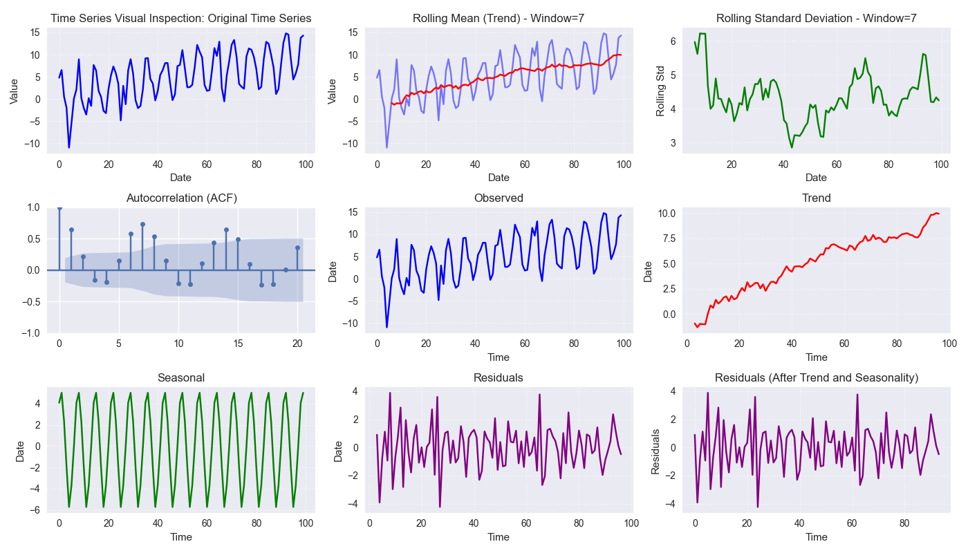
Plot visual panels for time-series analysis including decomposition.

get_decomposition_method

API Reference:

get_decomposition_method()

Purpose: To provide a heuristic estimate of a suitable decomposition model type (‘additive’ or ‘multiplicative’) and a basic guess for the seasonal period.

Functionality:

1. Takes DataFrame df, value_col.

2. Method Inference (`method=’auto’`): Suggests ‘multiplicative’ if all values > 0, otherwise suggests ‘additive’. Can be overridden.

3. Period Inference: Uses very basic logic (returns 1 or min_period). Not reliable for finding true seasonality.

Usage Context: A quick, rule-based first guess for decomposition parameters, mainly distinguishing additive/multiplicative based on positivity. Limited utility for period detection.

Code Example:

import pandas as pd
from fusionlab.utils.ts_utils import get_decomposition_method

# Data with positive values
df_pos = pd.DataFrame({'Value': [10, 12, 15, 13]})
method1, period1 = get_decomposition_method(df_pos, 'Value', method='auto')
print(f"Positive Data -> Method: {method1}, Period: {period1}")
# Expected: multiplicative, 1 (or min_period)

# Data with non-positive values
df_nonpos = pd.DataFrame({'Value': [10, -2, 15, 0]})
method2, period2 = get_decomposition_method(df_nonpos, 'Value', method='auto')
print(f"Non-Positive Data -> Method: {method2}, Period: {period2}")
# Expected: additive, 1 (or min_period)

infer_decomposition_method

API Reference:

infer_decomposition_method()

Purpose: To determine the more appropriate decomposition method (‘additive’ or ‘multiplicative’) using either a positivity heuristic or by comparing residual variances from both decomposition types.

Functionality:

Takes df, dt_col, required period.

1. `method=’heuristic’`: Checks if all values > 0. Returns ‘multiplicative’ or ‘additive’.

2. `method=’variance_comparison’`: Performs both additive and multiplicative decomposition (statsmodels) using the given period. Calculates residual variance (\(Var(\epsilon_t)\)) for both. Returns the method (‘additive’/’multiplicative’) with the lower residual variance. Optionally plots residual histograms (view=True) or returns components (return_components=True).

Usage Context: A more data-driven approach (variance comparison) than the simple heuristic for choosing between models, assuming the correct period is known. Requires statsmodels.

Code Example:

import numpy as np
import pandas as pd
# Assuming infer_decomposition_method is importable
from fusionlab.utils.ts_utils import infer_decomposition_method

# Create dummy data (e.g., additive seasonality)
dates = pd.date_range('2020-01-01', periods=48, freq='MS')
trend = np.linspace(50, 100, 48)
seasonal = 10 * np.sin(2 * np.pi * dates.month / 12)
noise = np.random.randn(48) * 2
values = trend + seasonal + noise
df = pd.DataFrame({'Date': dates, 'Value': values})

# Infer method using variance comparison (requires period)
seasonal_period = 12
best_method = infer_decomposition_method(
    df,
    dt_col='Date',
    value_col= 'Value', # value col must be specified as kwarg argument
    period=seasonal_period,
    method='variance_comparison',
    view=False # Set True to see plots
)
print(f"--- Decomposition Method Inference ---")
print(f"Data designed as additive.")
print(f"Best method by variance comparison: '{best_method}'")
# Expected: Often 'additive' for this data, but noise can influence

Expected Output:

Decomposition method inferred.

decompose_ts

API Reference:

decompose_ts()

Purpose: To perform time series decomposition, separating a series (value_col) into Trend (\(T_t\)), Seasonal (\(S_t\)), and Residual (\(R_t\)) components using statsmodels methods (STL or classical SDT).

Functionality:

1. Takes df, value_col, optional dt_col, method (‘additive’ or ‘multiplicative’ for SDT), strategy (‘STL’ or ‘SDT’), seasonal_period.

2. Selects Algorithm:

   • ‘STL’: Uses statsmodels.tsa.seasonal.STL (robust, flexible).

   • ‘SDT’: Uses statsmodels.tsa.seasonal.seasonal_decompose (classical additive/multiplicative).

3. Performs decomposition using the specified seasonal_period.

4. Returns input DataFrame augmented with ‘trend’, ‘seasonal’, and ‘residual’ columns.

Mathematical Models:

• Additive: \(Y_t = T_t + S_t + R_t\)

• Multiplicative: \(Y_t = T_t \times S_t \times R_t\)

Usage Context: Explicitly extracts and adds decomposition components to your DataFrame for analysis, visualization, separate forecasting, or use as features. Requires statsmodels.

Code Example:

import numpy as np
import pandas as pd
from fusionlab.utils.ts_utils import decompose_ts

# Create dummy data (use data from infer_decomposition_method)
dates = pd.date_range('2020-01-01', periods=48, freq='MS')
trend = np.linspace(50, 100, 48)
seasonal = 10 * np.sin(2 * np.pi * dates.month / 12)
noise = np.random.randn(48) * 2
values = trend + seasonal + noise
df = pd.DataFrame({'Date': dates, 'Value': values})

# Decompose using STL (additive is implicit for STL)
seasonal_period = 12
df_decomposed_stl = decompose_ts(
    df,
    value_col='Value',
    dt_col='Date',
    strategy='STL', # Specify STL strategy
    seasonal_period=seasonal_period
)

print("--- STL Decomposition Output ---")
print(df_decomposed_stl[['Value', 'trend', 'seasonal', 'residual']].head())

# Decompose using classical SDT (additive)
df_decomposed_sdt = decompose_ts(
    df,
    value_col='Value',
    dt_col='Date',
    strategy='SDT', # Specify classical strategy
    method='additive', # Specify model type
    seasonal_period=seasonal_period
)
print("\n--- SDT (Additive) Decomposition Output ---")
print(df_decomposed_sdt[['Value', 'trend', 'seasonal', 'residual']].head())

transform_stationarity

API Reference:

transform_stationarity()

Purpose: To apply common transformations aimed at achieving or improving time series stationarity (stabilizing mean/variance).

Functionality:

Applies a transformation to value_col based on method:

• ‘differencing’: Applies differencing of order or uses seasonal_period. \(\nabla Y_t = Y_t - Y_{t-1}\).

• ‘log’: Applies \(\ln(Y_t)\) (requires \(Y_t > 0\)).

• ‘sqrt’: Applies \(\sqrt{Y_t}\) (requires \(Y_t \ge 0\)).

• `’detrending’`: Removes trend using:

  • ‘linear’: Subtracts OLS linear fit \(Y_t - (\beta_0 + \beta_1 t)\).

  • ‘stl’: Returns residual component \(R_t\) from STL decomposition.

Adds transformed series as '<value_col>_transformed'. Optionally drops original (drop_original) or plots (view).

Usage Context: Preprocessing step for models assuming stationarity (e.g., ARIMA). Use differencing for trends/seasonality, log/sqrt for variance stabilization. Requires statsmodels for STL detrending.

Code Example:

import numpy as np
import pandas as pd
from fusionlab.utils.ts_utils import transform_stationarity

# Create dummy data with upward trend
dates = pd.date_range('2023-01-01', periods=50)
values_up = np.linspace(10, 50, 50)**1.5 # Non-linear trend
df_up = pd.DataFrame({'Date': dates, 'Value': values_up})
df_up['Date'] = pd.to_datetime(df_up['Date']) # Ensure datetime
df_up.set_index('Date', inplace=True)

# Apply first-order differencing
df_diff = transform_stationarity(
    df_up.copy(), # Use copy
    value_col='Value',
    method='differencing',
    order=1,
    view=False
)
print("--- Differencing Output ---")
print(df_diff[['Value_transformed']].head()) # Note NaNs

# Apply log transform (add offset if data can be zero)
df_log = transform_stationarity(
    df_up.copy() + 0.01, # Ensure positive for log
    value_col='Value',
    method='log',
    view=False
)
print("\n--- Log Transform Output ---")
print(df_log[['Value_transformed']].head())

# Apply linear detrending
df_detrend = transform_stationarity(
    df_up.copy(),
    value_col='Value',
    method='detrending',
    detrend_method='linear',
    view=True
)
print("\n--- Linear Detrending Output ---")
print(df_detrend[['Value_transformed']].head())

Expected Output:

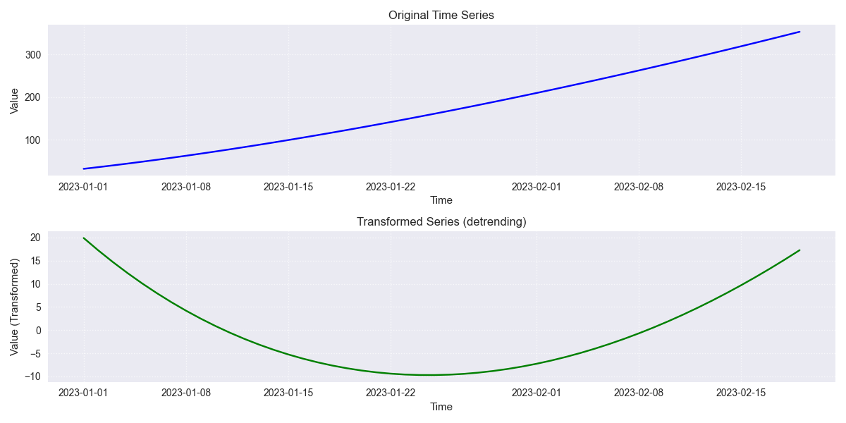
Stationary transformed plot.

ts_corr_analysis

API Reference:

ts_corr_analysis()

Purpose: To analyze and visualize time series correlations: autocorrelation (ACF), partial autocorrelation (PACF), and cross-correlation with external features.

Functionality:

1. ACF/PACF: Optional plots (view_acf_pacf=True) using statsmodels. ACF: \(\rho(h) = \frac{Cov(Y_t, Y_{t-h})}{\dots}\). Helps identify MA/AR orders for ARIMA.

2. Cross-Correlation: Calculates Pearson correlation (zero-lag) between value_col and specified features using scipy.stats.pearsonr. Optionally plots results (view_cross_corr=True).

3. Output: Returns dict with cross-correlation coefficients/p-values.

Usage Context: EDA tool to understand series memory (ACF/PACF) and identify potential external predictors (cross-correlation). Requires statsmodels, scipy, matplotlib.

Code Example (Results Only):

import pandas as pd
from fusionlab.utils.ts_utils import ts_corr_analysis

# Dummy data with target and feature
dates = pd.date_range('2023-01-01', periods=50)
data = {
    'Date': dates,
    'Sales': 50 + np.arange(50)*0.5 + np.random.randn(50)*5,
    'Promo': np.random.randint(0, 2, 50)
}
df = pd.DataFrame(data)

# Perform analysis, get results dict (suppress plots)
results = ts_corr_analysis(
    df,
    dt_col='Date',
    value_col='Sales',
    lags=10, # Lags for ACF/PACF calculation (if viewed)
    features=['Promo'], # Check correlation with Promo
    view_acf_pacf=True, # False to suppress ACF/PACF plots
    view_cross_corr=False # Suppress cross-corr plot
)

print("--- Correlation Analysis Results ---")
print("Cross-Correlation with 'Promo':")
print(results['cross_corr'])
# Note: ACF/PACF values are not returned, only plotted if view=True

Expected Output:

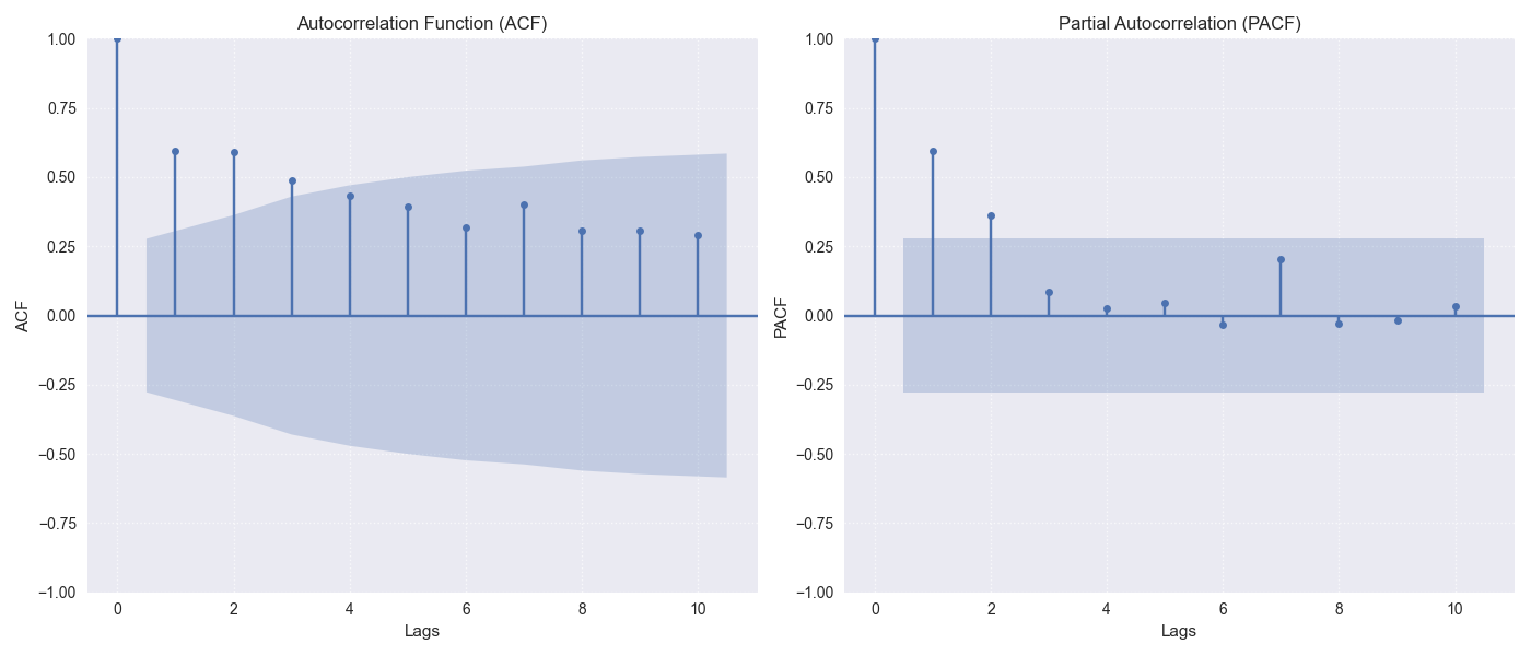
Time-Series Correlation Analysis

---

Feature Engineering

These utilities focus on creating new features from time series data that can be beneficial for machine learning models, capturing temporal dependencies, calendar effects, and other patterns.

ts_engineering

API Reference:

ts_engineering()

Purpose: To automatically generate a variety of common and useful time series features from a DataFrame, augmenting it with predictors that capture temporal dynamics, seasonality, and other patterns.

Functionality: Takes a DataFrame df (with a datetime index or dt_col), the primary value_col, and various parameters:

1. Time-Based Features: Extracts year, month, day, day_of_week, is_weekend, quarter, hour.

2. Holiday Indicator: Creates binary ‘is_holiday’ if holiday_df provided.

3. Lag Features: Creates lags number of lag features (e.g., \(Y_{t-1}, Y_{t-2}\)).

4. Rolling Statistics: Calculates rolling mean/std dev over window size (\(W\)).

   \[\begin{split}\text{RollingMean}_t = \frac{1}{W}\sum_{i=0}^{W-1} Y_{t-i} \\ \text{RollingStd}_t = \sqrt{\frac{1}{W-1}\sum_{i=0}^{W-1} (Y_{t-i} - \text{RollingMean}_t)^2}\end{split}\]

5. Differencing: Creates differenced series of diff_order (\(\nabla Y_t = Y_t - Y_{t-1}\) for order 1).

6. Seasonal Differencing: Optional differencing at seasonal_period lag \(S\) (\(Y_t - Y_{t-S}\)).

7. Fourier Features: Optional FFT magnitude features (apply_fourier=True).

8. NA Handling: Fills NaNs from lags/rolling/diff using ffill, then drops remaining.

9. Scaling: Optional scaling of numeric features (scaler=’z-norm’ or ‘minmax’).

Usage Context: A powerful utility for automating the creation of a rich feature set for time series models. The resulting DataFrame can be used directly or passed to sequence preparation utilities like create_sequences() or reshape_xtft_data().

Code Example:

import pandas as pd
import numpy as np
# Assuming ts_engineering is importable
from fusionlab.utils.ts_utils import ts_engineering

# Create dummy data
dates = pd.date_range('2023-01-01', periods=20)
df = pd.DataFrame({'Date': dates, 'Value': np.arange(20) * 2.5 + 10})
df = df.set_index('Date') # Use datetime index

# Apply feature engineering
df_featured = ts_engineering(
    df=df.copy(), # Pass a copy
    value_col='Value',
    lags=2,
    window=3,
    diff_order=1,
    scaler='z-norm' # Apply scaling at the end
)

print("--- Engineered Features ---")
print("Columns:", df_featured.columns.tolist())
print("\nHead (Note NaNs from lags/rolling/diff & scaling):")
print(df_featured.head())

create_lag_features

API Reference:

create_lag_features()

Purpose: To generate lagged features for one or more specified time series columns in a DataFrame. Lag features represent past values and are fundamental predictors for many time series models.

Functionality:

1. Takes df, value_col, optional dt_col, optional list lag_features, and list of integer lags.

2. Ensures datetime index (using ts_validator).

3. For each specified feature and lag interval \(k\) in lags, creates a new column <feature>_lag_<k> by shifting the original column down by \(k\) steps.

   \[\text{Feature}_{lag\_k}(t) = \text{Feature}(t-k)\]

4. Optionally includes original columns (include_original).

5. Optionally drops rows with NaNs created by shifting (dropna).

6. Optionally resets the index (reset_index).

Usage Context: A core feature engineering step. Use this function when you specifically need to create lag features for one or more columns. For a broader range of features (rolling stats, time features, etc.), consider ts_engineering().

Code Example:

import pandas as pd
import numpy as np
from fusionlab.utils.ts_utils import create_lag_features

# Create dummy data
dates = pd.date_range('2023-01-01', periods=10)
df = pd.DataFrame({
    'Date': dates,
    'Value': np.arange(10) + 5,
    'Other': np.arange(10) * 2 + 3
})
df = df.set_index('Date')

# Create lags 1 and 2 for 'Value' column
df_lagged = create_lag_features(
    df.copy(),
    value_col='Value',
    lags=[1, 2],
    dropna=False, # Keep NaNs initially
    include_original=True,
    reset_index=False # Keep datetime index
)

print("--- DataFrame with Lag Features ---")
print(df_lagged.head())

# Example dropping NaNs
df_lagged_dropped = create_lag_features(
    df.copy(), value_col='Value', lags=[1, 2], dropna=True
)
print("\n--- DataFrame with Lags (NaNs Dropped) ---")
print(df_lagged_dropped.head())

---

Feature Selection & Reduction

After potentially generating many features (e.g., via lags, rolling stats, etc.), these utilities can help select the most relevant ones or reduce the dimensionality of the feature space.

select_and_reduce_features

API Reference:

select_and_reduce_features()

Purpose: To perform feature selection by removing highly correlated features or reduce dimensionality using Principal Component Analysis (PCA).

Functionality: Takes df, optional target_col/exclude_cols. Operates based on method:

• method=’corr’: Removes features highly correlated with others.

  1. Calculates pairwise Pearson correlation matrix for numeric features.

  2. Identifies pairs exceeding corr_threshold.

  3. Drops one feature from each highly correlated pair.

• method=’pca’: Uses Principal Component Analysis.

  1. Optionally standardizes features (scale_data=True). Requires scikit-learn.

  2. Applies sklearn.decomposition.PCA to keep n_components (either an int count or a float variance ratio).

  3. Replaces original features with principal components (PCs).

  \[\text{ExplainedVarianceRatio}(PC_i) = \frac{\lambda_i}{\sum_j \lambda_j}\]

  where \(\lambda_i\) are eigenvalues.

Returns transformed DataFrame (optionally with target). Can also return the fitted PCA model (return_pca=True).

Usage Context: Use after extensive feature engineering (ts_engineering()) to combat multicollinearity (method=’corr’) or reduce feature dimensions (method=’pca’) before model training. Requires scikit-learn for PCA.

Code Examples:

Example 1: Correlation-Based Selection

import pandas as pd
import numpy as np
from fusionlab.utils.ts_utils import select_and_reduce_features

# Dummy data with correlated features
data = {
    'A': np.arange(10),
    'B': np.arange(10) * 1.05 + np.random.randn(10)*0.1, # Highly correlated with A
    'C': np.random.randn(10), # Uncorrelated
    'Target': np.random.randint(0, 2, 10)
}
df = pd.DataFrame(data)
print("--- Original Columns ---")
print(df.columns.tolist())

# Select features, removing those with >0.95 correlation
df_selected = select_and_reduce_features(
    df.copy(),
    target_col='Target',
    method='corr',
    corr_threshold=0.95
)
print("\n--- Columns after Correlation Selection ---")
print(df_selected.columns.tolist()) # Should drop 'B'

Example 2: PCA Reduction

import pandas as pd
import numpy as np
# Assuming select_and_reduce_features is importable
from fusionlab.utils.ts_utils import select_and_reduce_features

# Use same dummy data
data = {
    'A': np.arange(10), 'B': np.arange(10) * 1.05,
    'C': np.random.randn(10), 'Target': np.random.randint(0, 2, 10)
}
df = pd.DataFrame(data)

# Reduce features A, B, C to 2 principal components
df_pca, pca_model = select_and_reduce_features(
    df.copy(),
    target_col='Target',
    method='pca',
    n_components=2, # Keep top 2 components
    scale_data=True, # Recommended for PCA
    return_pca=True
)
print("\n--- DataFrame after PCA Reduction ---")
print(df_pca.head())
print("\nExplained Variance Ratio per component:")
print(pca_model.explained_variance_ratio_)

---