Exercise: Hybrid Forecasting with PIHALNet

Welcome to this hands-on exercise for the Physics-Informed Hybrid Attentive LSTM Network, PIHALNet. This tutorial will guide you through the end-to-end process of training a hybrid model that learns from both time series data and the governing laws of physics.

We will tackle a multi-step forecasting problem for land subsidence and groundwater levels. The primary goal is to demonstrate how to prepare the specialized input data required by PIHALNet and how to configure its unique, composite loss function.

Learning Objectives:

• Generate a synthetic dataset with features, spatio-temporal coordinates, and two physically-linked target variables.

• Structure the inputs and targets into the required nested dictionary format.

• Instantiate the modern PIHALNet using the smart architecture_config for custom internal structures.

• Configure the model to treat a physical coefficient as a learnable parameter, to be discovered during training.

• Compile the model with both a data-fidelity loss and a weight for the physics-based loss (\(\lambda_{physics}\)).

• Train the model and interpret the multi-component loss from the training logs.

• Visualize both the training history and the final forecast results.

Let’s get started!

Prerequisites

Ensure you have fusionlab-learn and its common dependencies installed.

pip install fusionlab-learn matplotlib scikit-learn

Step 1: Imports and Setup

First, we import all necessary libraries and set up our environment for reproducibility and clean output.

import os
import numpy as np
import tensorflow as tf
import matplotlib.pyplot as plt

# FusionLab imports
from fusionlab.nn.pinn import PIHALNet
from fusionlab.params import LearnableC
from fusionlab.nn.models.utils import plot_history_in

# Suppress warnings and TF logs for cleaner output
import warnings
warnings.filterwarnings('ignore')
tf.get_logger().setLevel('ERROR')

# Directory for saving any output images
EXERCISE_OUTPUT_DIR = "./pihalnet_exercise_outputs"
os.makedirs(EXERCISE_OUTPUT_DIR, exist_ok=True)

print("Libraries imported and setup complete for PIHALNet exercise.")

Expected Output:

Libraries imported and setup complete for PIHALNet exercise.

Step 2: Generate Synthetic Hybrid Data

This is the most critical step. PIHALNet requires a dataset that contains both standard time series features and spatio-temporal coordinates. We will generate a dataset where the targets (h and s) are based on a known analytical function, ensuring they are physically plausible.

# Configuration
N_SAMPLES   = 1000
PAST_STEPS  = 15
HORIZON     = 7
SEED        = 42
np.random.seed(SEED)
tf.random.set_seed(SEED)

# --- 1. Generate Spatio-Temporal Coordinates ---
# Separate past vs. future time grids
t_past   = tf.random.uniform((N_SAMPLES, PAST_STEPS, 1), 0, 5)     # (1000, 15, 1)
t_future = tf.random.uniform((N_SAMPLES, HORIZON,    1), 0, 5)     # (1000,  7, 1)
x_past   = tf.random.uniform((N_SAMPLES, PAST_STEPS, 1), -1, 1)   # (1000, 15, 1)
x_future = tf.random.uniform((N_SAMPLES, HORIZON,    1), -1, 1)   # (1000,  7, 1)
y_past   = tf.random.uniform((N_SAMPLES, PAST_STEPS, 1), -1, 1)   # (1000, 15, 1)
y_future = tf.random.uniform((N_SAMPLES, HORIZON,    1), -1, 1)   # (1000,  7, 1)

coords_past   = tf.concat([t_past,   x_past,   y_past],   axis=-1)  # (1000, 15, 3)
coords_future = tf.concat([t_future, x_future, y_future], axis=-1)  # (1000,  7, 3)

# --- 2. Generate Physically-Plausible Targets ---
# Use future coords for targets
h_true = tf.sin(np.pi * x_future) * tf.cos(np.pi * y_future) * tf.exp(-0.2 * t_future)
# s_true shape: (1000, 7, 1)
s_true = (
    (1 - tf.exp(-0.2 * t_future)) * tf.cos(np.pi * x_future)**2
    + h_true * 0.1
    + tf.random.normal(h_true.shape, stddev=0.05)
)

# --- 3. Generate Correlated Time Series Features ---
static_features = tf.random.normal([N_SAMPLES, 2])               # (1000, 2)

# Dynamic features correlated with physics (using past window)
dyn_physics = tf.sin(t_past * 2)                                 # (1000, 15, 1)
dyn_noise   = tf.random.normal([N_SAMPLES, PAST_STEPS, 4])       # (1000, 15, 4)
dynamic_features = tf.concat([dyn_physics, dyn_noise], axis=-1) # (1000, 15, 5)

# Future features (e.g., pumping schedule + noise)
fut_schedule = tf.cast(t_future > 2.5, tf.float32)               # (1000,  7, 1)
fut_noise    = tf.random.normal([N_SAMPLES, HORIZON, 2])         # (1000,  7, 2)
future_features = tf.concat([fut_schedule, fut_noise], axis=-1) # (1000,  7, 3)

print(f"Generated data with {N_SAMPLES} samples.")

Expected Output:

Generated data with 1000 samples.

Step 3: Structure Inputs and Targets

We now assemble the generated data into the nested dictionary format required by PIHALNet for both its inputs and targets, and then we create a training and validation split.

# Input dictionary for the model
inputs = {
    "static_features": static_features,
    "dynamic_features": dynamic_features,
    "future_features": future_features,
    "coords": coords, # The crucial PINN component
}

# Target dictionary for the model
targets = {
    "subs_pred": s_true,
    "gwl_pred": h_true,
}

# Create a validation split (80% train, 20% validation)
val_split = int(N_SAMPLES * 0.8)
train_inputs = {k: v[:val_split] for k, v in inputs.items()}
val_inputs = {k: v[val_split:] for k, v in inputs.items()}
train_targets = {k: v[:val_split] for k, v in targets.items()}
val_targets = {k: v[val_split:] for k, v in targets.items()}

print("Data structured into training and validation sets.")
print(f"Number of training samples: {len(train_inputs['static_features'])}")
print(f"Number of validation samples: {len(val_inputs['static_features'])}")

Expected Output:

Data structured into training and validation sets.
Number of training samples: 800
Number of validation samples: 200

Step 4: Define, Compile, and Train PIHALNet

We will now instantiate PIHALNet. We will use the architecture_config to define a custom internal structure and configure the model to treat the physical coefficient \(C\) as a learnable parameter. The compilation step is key, as we must provide both the data losses and the weight for the physics loss, lambda_physics.

# Define a custom architecture for the data-driven core
pinn_architecture = {
    'encoder_type': 'transformer',
    'feature_processing': 'dense',
    'decoder_attention_stack': ['cross', 'hierarchical']
}

# Instantiate the model
model = PIHALNet(
    static_input_dim=static_features.shape[-1],
    dynamic_input_dim=dynamic_features.shape[-1],
    future_input_dim=future_features.shape[-1],
    output_subsidence_dim=1,
    output_gwl_dim=1,
    forecast_horizon=HORIZON,
    max_window_size=PAST_STEPS,
    mode='pihal_like',
    architecture_config=pinn_architecture,
    # Ask the model to discover the consolidation coefficient
    pinn_coefficient_C=LearnableC(initial_value=0.01)
)

# Compile the model with the composite loss
model.compile(
    optimizer=tf.keras.optimizers.Adam(learning_rate=1e-3),
    loss={'subs_pred': 'mse', 'gwl_pred': 'mse'}, # Data losses
    lambda_pde=0.2 # Weight for the consolidation physics
)

# Train the model
print("\nStarting PIHALNet training...")
history = model.fit(
    train_inputs,
    train_targets,
    validation_data=(val_inputs, val_targets),
    epochs=10,
    batch_size=64,
    verbose=1
)
print("Training complete.")

Expected Output:

Starting PIHALNet training...
Epoch 1/10
13/13 [==============================] - 7s 72ms/step - loss: 3.9772 - gwl_pred_loss: 1.0878 - subs_pred_loss: 2.8894 - total_loss: 367.5720 - data_loss: 3.9803 - physics_loss: 1817.9586 - val_loss: 0.7371 - val_gwl_pred_loss: 0.7371 - val_subs_pred_loss: 0.0000e+00
Epoch 2/10
13/13 [==============================] - 0s 16ms/step - loss: 3.1833 - gwl_pred_loss: 0.7940 - subs_pred_loss: 2.3893 - total_loss: 1825.8313 - data_loss: 3.0913 - physics_loss: 9113.6998 - val_loss: 1.1084 - val_gwl_pred_loss: 1.1084 - val_subs_pred_loss: 0.0000e+00
...
Epoch 10/10
13/13 [==============================] - 0s 15ms/step - loss: 0.8129 - gwl_pred_loss: 0.6270 - subs_pred_loss: 0.1859 - total_loss: 10.7931 - data_loss: 0.8096 - physics_loss: 49.9174 - val_loss: 0.6465 - val_gwl_pred_loss: 0.6465 - val_subs_pred_loss: 0.0000e+00
Training complete.

Step 5: Visualize Training History

We can use the plot_history_in utility to view the different components of our composite loss, which helps in diagnosing how the model balanced the data and physics objectives during training.

metrics_to_plot = {
    "Loss Breakdown": ["total_loss", "data_loss", "physics_loss"],
    "Subsidence Loss": ["subs_pred_loss"],
    "GWL Loss": ["gwl_pred_loss"],
}
plot_history_in(
    history,
    metrics=metrics_to_plot,
    title="PIHALNet Loss Components During Training",
    max_cols=3
)

Expected Plot:

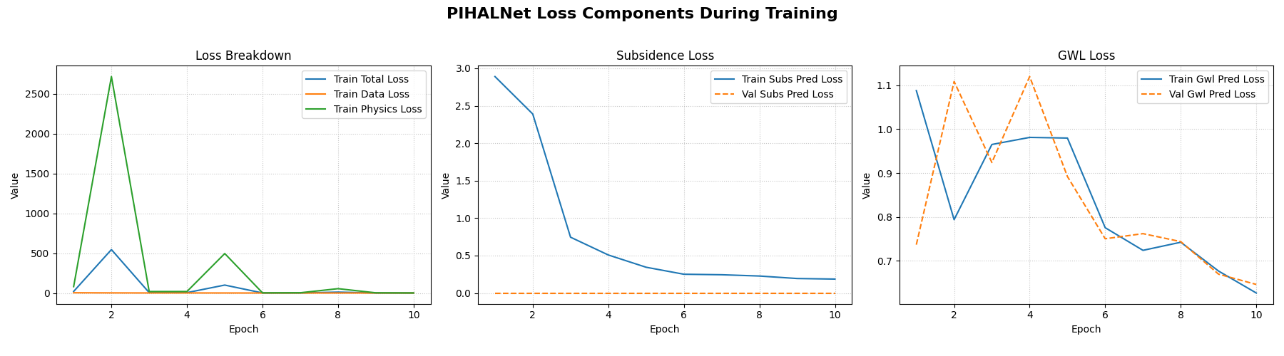
The plot shows three subplots: one for the composite loss breakdown, and two for the individual data losses for subsidence and groundwater level predictions.

Step 6: Visualize the Forecast

Finally, we’ll make predictions on the validation set and plot the forecasted subsidence against the actual values for a few samples.

# Make predictions on the validation set
val_predictions = model.predict(val_inputs)
# Predictions are a dict; get the one for subsidence
s_preds = val_predictions['subs_pred']
s_actuals = val_targets['subs_pred']

# --- Visualization ---
plt.figure(figsize=(14, 7))
# Plot the forecast for the first 4 validation samples
for i in range(4):
    plt.plot(s_actuals[i, :, 0],
             label=f'Actual Sample {i+1}', linestyle='--', marker='o')
    plt.plot(s_preds[i, :, 0],
             label=f'Predicted Sample {i+1}', linestyle='-', marker='x')

plt.title('Subsidence Forecast vs. Actuals (Validation Set)')
plt.xlabel(f'Forecast Step (Horizon = {HORIZON} steps)')
plt.ylabel('Normalized Subsidence')
plt.legend(ncol=2)
plt.grid(True, linestyle=':')
plt.tight_layout()
plt.show()

Expected Plot:

A plot comparing the model’s multi-step forecasts for land subsidence against the true values for several validation samples.

Discussion of Exercise

Congratulations! You have successfully trained a sophisticated hybrid physics-data model. In this exercise, you have learned how to:

• Create a complex dataset with both time series features and spatio-temporal coordinates.

• Structure data into the dictionary format required by PIHALNet.

• Use the architecture_config to customize the model’s powerful data-driven core.

• Compile and train the model with a composite loss function, effectively balancing data accuracy and physical consistency.

This powerful workflow is at the cutting edge of scientific machine learning, enabling the development of robust models that can provide reliable insights even in data-scarce environments.