Exercise: Hybrid Forecasting with TransFlowSubsNet

Welcome to this exercise on using TransFlowSubsNet, a hybrid physics-informed neural network from the fusionlab-learn library. This model is unique because it learns from two sources of information simultaneously: structured time series data and the governing laws of physics.

We will perform a multi-step forecast for both groundwater level and land subsidence. This exercise will walk you through the specific data preparation needed to satisfy both the data-driven and physics-informed components of the model.

Learning Objectives:

• Generate a synthetic dataset with features, coordinates, and two target variables (subsidence and groundwater level).

• Structure the inputs into the required dictionary format, separating feature inputs from coordinate inputs.

• Instantiate TransFlowSubsNet with both data-driven and physics-informed configurations.

• Compile the model with a composite data loss and physics-loss weights (\(\lambda_{gw}\), \(\lambda_{c}\)).

• Train the model and interpret the multi-component loss in the training log.

• Visualize the forecast results against the true values.

Let’s begin!

Prerequisites

Ensure you have fusionlab-learn and its common dependencies installed.

pip install fusionlab-learn matplotlib

Step 1: Imports and Setup

First, we import all necessary libraries and set up our environment.

import os
import numpy as np
import tensorflow as tf
import matplotlib.pyplot as plt
import warnings

# FusionLab imports
from fusionlab.nn.pinn import TransFlowSubsNet
from fusionlab.nn.models.utils import plot_history_in

# Suppress warnings and TF logs for cleaner output
warnings.filterwarnings('ignore')
tf.get_logger().setLevel('ERROR')

# Directory for saving any output images
EXERCISE_OUTPUT_DIR = "./transflow_exercise_outputs"
os.makedirs(EXERCISE_OUTPUT_DIR, exist_ok=True)

print("Libraries imported and setup complete for TransFlowSubsNet exercise.")

Expected Output:

Libraries imported and setup complete for TransFlowSubsNet exercise.

Step 2: Generate Synthetic Hybrid Data

This is the most critical step. We need to create a dataset that includes: 1. Standard time series features (static, dynamic, future). 2. Spatio-temporal coordinates (t, x, y). 3. Two target variables (groundwater_level, subsidence) that are

logically linked to the coordinates and features.

# Configuration
N_SAMPLES = 500
PAST_STEPS = 12
HORIZON = 6
SEED = 42
np.random.seed(SEED)
tf.random.set_seed(SEED)

# --- Generate Coordinates ---
t = tf.random.uniform((N_SAMPLES, HORIZON, 1), 0, 10)
t_past = tf.random.uniform((N_SAMPLES, PAST_STEPS, 1), 0, 10)
x = tf.random.uniform((N_SAMPLES, HORIZON, 1), -1, 1)
y = tf.random.uniform((N_SAMPLES, HORIZON, 1), -1, 1)
coords = tf.concat([t, x, y], axis=-1)

# --- Generate Physically-Plausible Targets ---
# Groundwater level (h) based on a simple analytical solution
h_true = tf.sin(np.pi * x) * tf.cos(np.pi * y) * tf.exp(-0.1 * t)
# Subsidence (s) as an integrated function of head decline
s_true = (1 - tf.exp(-0.1 * t)) * (tf.cos(np.pi * x))**2 + h_true * 0.1

# --- Generate Correlated Features ---
# These features will be used by the data-driven part of the model
static_features = tf.random.normal([N_SAMPLES, 3])
# Dynamic features correlated with the physics
dynamic_features = tf.concat([
    tf.sin(t_past[:, :PAST_STEPS, :]),
    tf.random.normal([N_SAMPLES, PAST_STEPS, 7])
], axis=-1)
# Future features
future_features = tf.random.normal([N_SAMPLES, HORIZON, 4])

print("Generated data shapes:")
print(f"  Static Features:  {static_features.shape}")
print(f"  Dynamic Features: {dynamic_features.shape}")
print(f"  Future Features:  {future_features.shape}")
print(f"  Coordinates:      {coords.shape}")
print(f"  True GWL Target:    {h_true.shape}")
print(f"  True Subsidence Target: {s_true.shape}")

Expected Output:

Generated data shapes:
  Static Features:  (500, 3)
  Dynamic Features: (500, 12, 8)
  Future Features:  (500, 6, 4)
  Coordinates:      (500, 6, 3)
  True GWL Target:    (500, 6, 1)
  True Subsidence Target: (500, 6, 1)

Step 3: Structure Inputs and Targets for Training

TransFlowSubsNet expects a dictionary of inputs and a dictionary of targets for its .fit() method. We now assemble the data we generated into this required format.

# Input dictionary for the model
inputs = {
    "static_features": static_features,
    "dynamic_features": dynamic_features,
    "future_features": future_features,
    "coords": coords, # The crucial PINN component
}

# Target dictionary for the model
targets = {
    "subs_pred": s_true,
    "gwl_pred": h_true,
}

# Create a validation split
val_split = int(N_SAMPLES * 0.8)
train_inputs = {k: v[:val_split] for k, v in inputs.items()}
val_inputs = {k: v[val_split:] for k, v in inputs.items()}
train_targets = {k: v[:val_split] for k, v in targets.items()}
val_targets = {k: v[val_split:] for k, v in targets.items()}

print("Data structured into training and validation sets.")

Step 4: Define, Compile, and Train TransFlowSubsNet

We now instantiate the model. The most important step is .compile(), where we provide both the standard data loss functions (one for each target) and the weights for the physics-based losses (\(\lambda_{gw}\) and \(\lambda_{c}\)).

# Instantiate the model
model = TransFlowSubsNet(
    static_input_dim=static_features.shape[-1],
    dynamic_input_dim=dynamic_features.shape[-1],
    future_input_dim=future_features.shape[-1],
    output_subsidence_dim=1,
    output_gwl_dim=1,
    forecast_horizon=HORIZON,
    max_window_size=PAST_STEPS,
    mode='pihal_like',
    pde_mode='both',      # Use both physics loss terms
    K='learnable',        # Ask the model to infer K
    pinn_coefficient_C=0.01 # Use a fixed C
)

# Compile the model with composite loss
model.compile(
    optimizer=tf.keras.optimizers.Adam(learning_rate=1e-3),
    loss={'subs_pred': 'mse', 'gwl_pred': 'mse'}, # Data losses
    lambda_gw=1.0,      # Weight for groundwater physics
    lambda_cons=0.5     # Weight for consolidation physics
)

# Train the model
print("\nStarting TransFlowSubsNet training...")
history = model.fit(
    train_inputs,
    train_targets,
    validation_data=(val_inputs, val_targets),
    epochs=5,
    batch_size=32,
    verbose=1
)
print("Training complete.")

Expected Output:

Starting TransFlowSubsNet training...
Epoch 1/5
13/13 [==============================] - 37s 237ms/step - loss: 1.0443 - gwl_pred_loss: 0.6407 - subs_pred_loss: 0.4036 - total_loss: 0.9620 - data_loss: 0.9616 - consolidation_loss: 8.8173e-04 - gw_flow_loss: 1.6358e-07 - val_loss: 0.1779 - val_gwl_pred_loss: 0.1779 - val_subs_pred_loss: 0.0000e+00
Epoch 2/5
13/13 [==============================] - 0s 24ms/step - loss: 0.2164 - gwl_pred_loss: 0.1499 - subs_pred_loss: 0.0665 - total_loss: 0.2129 - data_loss: 0.2128 - consolidation_loss: 2.9616e-04 - gw_flow_loss: 4.7181e-08 - val_loss: 0.1271 - val_gwl_pred_loss: 0.1271 - val_subs_pred_loss: 0.0000e+00
...
Epoch 5/5
13/13 [==============================] - 0s 24ms/step - loss: 0.1502 - gwl_pred_loss: 0.1120 - subs_pred_loss: 0.0382 - total_loss: 0.1496 - data_loss: 0.1496 - consolidation_loss: 2.7363e-05 - gw_flow_loss: 7.7033e-10 - val_loss: 0.1170 - val_gwl_pred_loss: 0.1170 - val_subs_pred_loss: 0.0000e+00
Training complete.

Step 5: Visualize Training History

We can use the plot_history_in utility to view all the components of our composite loss function, which helps in understanding how the model balanced the data and physics objectives.

metrics_to_plot = {
    "Loss Breakdown": ["total_loss", "data_loss"],
    "Physics Residuals": ["consolidation_loss", "gw_flow_loss"]
}
plot_history_in(
    history,
    metrics=metrics_to_plot,
    title="TransFlowSubsNet Loss Components"
)

Expected Plot:

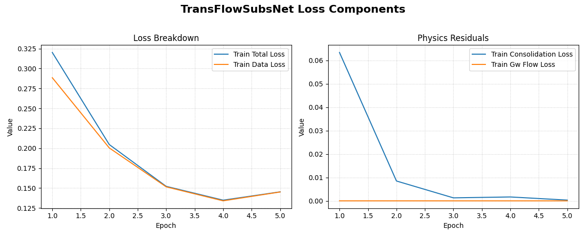
The plot shows two subplots: one comparing the total loss to the data-fidelity loss, and another showing the evolution of the two physics-based loss components.

Step 6: Visualize the Forecast

Finally, let’s make predictions on the validation set and compare the forecasted groundwater level against the actual values for a sample.

# Make predictions on the validation set
val_predictions = model.predict(val_inputs)
# Predictions are a dict, get the one for groundwater level
gwl_preds = val_predictions['gwl_pred']
gwl_actuals = val_targets['gwl_pred']

# Plot the forecast for the first 5 validation samples
plt.figure(figsize=(14, 7))
for i in range(5):
    plt.plot(gwl_actuals[i, :, 0],
             label=f'Actual Sample {i+1}', linestyle='--')
    plt.plot(gwl_preds[i, :, 0],
             label=f'Predicted Sample {i+1}', linestyle='-')

plt.title('Groundwater Level Forecast vs. Actuals (Validation Set)')
plt.xlabel(f'Forecast Step (Horizon = {HORIZON} steps)')
plt.ylabel('Normalized Groundwater Level')
plt.legend(ncol=2)
plt.grid(True, linestyle=':')
plt.tight_layout()
plt.show()

Expected Plot:

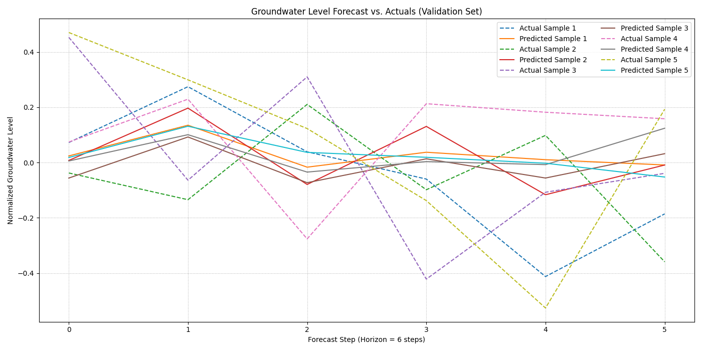
A comparison plot showing the model’s multi-step forecasts for the groundwater level against the true values for several validation samples.

Discussion of Exercise

Congratulations! You have successfully trained a hybrid physics-data model. In this exercise, you have learned to:

• Create a complex dataset suitable for a hybrid model that requires both feature and coordinate inputs.

• Structure the data into the dictionary format required by TransFlowSubsNet.

• Compile the model with a composite loss function, balancing data fidelity and physical consistency using loss weights.

• Train the model and interpret its multi-component loss log.

This workflow is a powerful paradigm for building more robust and generalizable scientific machine-learning models, especially in data-scarce or noisy environments where physics can provide a strong inductive bias.