Subsidence PINN Mini GUI Guide
This guide provides a complete walkthrough of the Subsidence PINN
Mini GUI, a desktop application designed to provide a user-friendly
interface for the complex forecasting workflows in fusionlab-learn.
The application allows users who may not be familiar with Python to load their own data, configure model parameters, run a full training and forecasting pipeline, and view the results, all from a simple graphical interface.

A preview of the main application window with its detailed configuration panels.
Launching the Application
The GUI is a tool within the fusionlab-learn library. To run it,
you must have the library and its dependencies (especially PyQt5)
installed.
Navigate to the root directory of the fusionlab-learn project in your terminal.
Run the application using the following command:
python -m fusionlab.tools.app.mini_forecaster_gui
This will launch the main application window.
User Interface Guide
The application is divided into several logical panels for configuration and results.
1. Data Input & Main Controls
These are the primary controls for managing the workflow.
Select CSV…: Click this button to open a file dialog. Navigate to and select the .csv file containing your spatiotemporal data. The filename will appear next to the button upon successful selection.
City / Dataset: This text field allows you to specify a name for your dataset (e.g., ‘zhongshan’, ‘nansha’). This name is used internally to manage configurations and to create uniquely named output directories for saving results, preventing runs from overwriting each other.
Run: Located at the bottom left, this button starts the end-to-end workflow using the current configuration. It becomes disabled while a process is running.
Reset: Located at the top right, this button clears all logs and results and resets all configuration options to their default values.
2. Data Preview and Editing
After a CSV file is selected, a new “Preview & Edit Data” button will appear. Clicking this opens a data preview window, allowing you to perform basic cleaning and preparation steps directly within the GUI before running the main workflow.
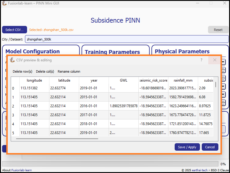
The data editor allows for quick modifications to the loaded dataset.
This window provides several useful tools:
Table Preview: Displays the first several rows of your dataset, allowing you to verify that it was loaded correctly.
Delete row(s): Allows you to select and remove specific rows from the dataset.
Delete col(s): Allows you to select and remove unwanted columns.
Rename column: Provides a dialog to rename a selected column.
Save / Apply: Saves all changes you’ve made and closes the window, updating the dataset that will be used by the main workflow.
Cancel: Closes the window without saving any changes.
3. Model Configuration
This panel allows you to configure the model’s core architecture.
Architecture: Choose between
TransFlowSubsNet(the advanced, coupled-physics model) andPIHALNet(the consolidation-focused model).Epochs: Sets the maximum number of training epochs.
Batch Size: Defines the number of samples processed in each batch during training.
Learning Rate: Sets the initial learning rate for the Adam optimizer.
Model Type: Sets the internal data handling mode, typically ‘pihal’ or ‘tft’.
Attention Levels: A comma-separated list defining which attention mechanisms to use (e.g., ‘1, 2, 3’).
Evaluate Coverage: A checkbox to enable the calculation of quantile coverage score after prediction.
4. Training Parameters
This panel controls the temporal aspects of the training and forecasting process.
Train End Year: The last year of data to be included in the training set.
Forecast Start Year: The first year for which predictions will be made.
Forecast Horizon (Years): The number of years to predict into the future.
Time Steps (look-back): The number of historical time steps to use as input for the model’s encoder.
Quantiles (comma-separated): A list of quantiles for probabilistic forecasting (e.g., 0.1, 0.5, 0.9). Leave blank for point forecasting.
5. Physical Parameters
This panel gives you fine-grained control over the physics-informed components.
Pinn Coeff C, K, Ss, Q: For each physical parameter, you can select
learnableto have the model infer its value, or provide a fixed numerical value.λ Consolidation / λ GW Flow: Sets the weights (\(\lambda_c\), \(\lambda_{gw}\)) for the physics loss terms.
PDE Mode: Controls which physics constraints are active during training (e.g., ‘both’, ‘consolidation’).
Weights (Subs. / GWL): Sets the relative importance of the data-fidelity loss for the two main targets (subsidence and groundwater level).
6. Feature Selection
This panel allows you to specify which columns from your input data should be used for the different feature streams.
Dyn. / Stat. / Future: Enter the names of your columns, separated by commas, into the appropriate fields for Dynamic, Static, and Future features. Leaving a field as
autowill let the application attempt to automatically detect the appropriate columns.
7. Log and Output Panel
The large text area at the bottom of the window is the Log Panel. This is your primary window into the workflow’s progress. It provides real-time, timestamped feedback for each major step, from data loading to model training and final visualization. Any warnings or errors that occur during the process will be printed here, providing crucial information for debugging.
Once the workflow is complete, this panel will also display the head of the final results DataFrame and any generated plots, giving you an immediate preview of the outcome.
8. Viewing the Results
Once the workflow finishes successfully, the GUI provides the results in two main ways: status updates on the main window and an interactive plot viewer.
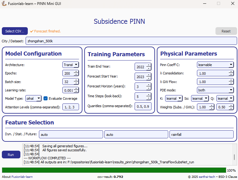
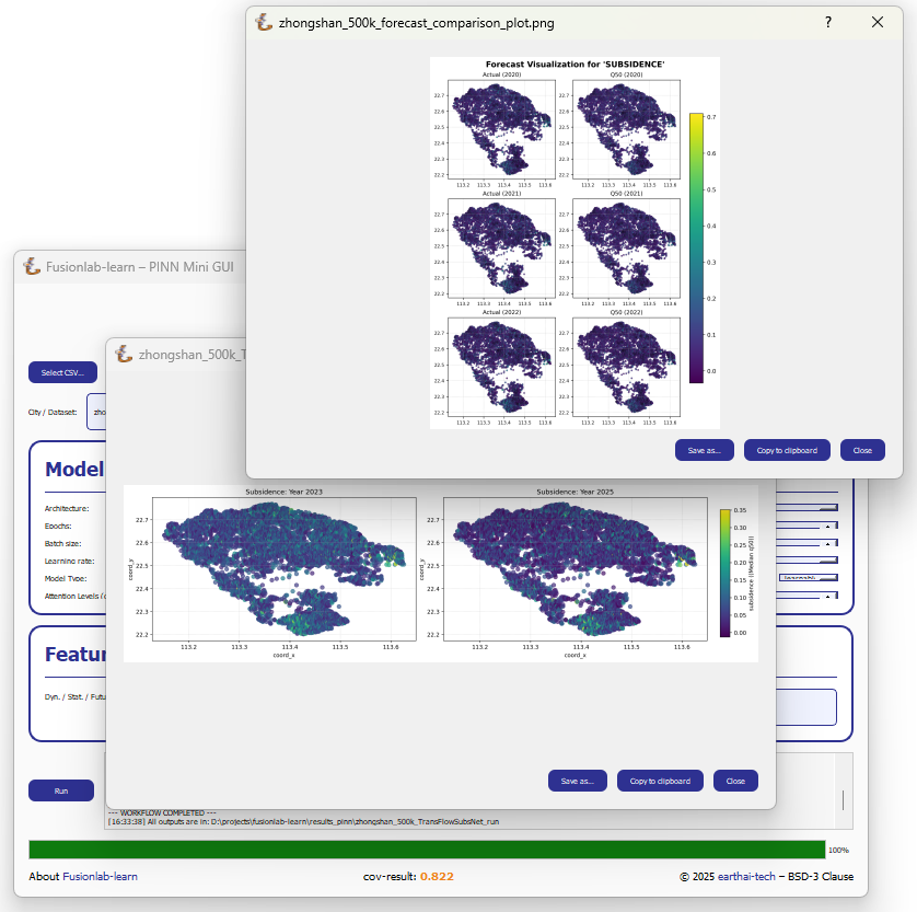
Main Window Updates (a): A checkmark and “Forecast finished” message appear at the top.If the “Evaluate Coverage” checkbox in the Model Configuration panel was ticked, the calculated coverage score (e.g., cov-result: 0.792) will be displayed in the bottom status bar.
Interactive Plot Viewer (b): A new window opens to display all plots generated during the run, such as the training history and forecast visualizations. This viewer allows you to inspect the visuals closely and provides options to “Save as…” or “Copy to clipboard” for easy export.
Final Log Messages: The log panel will show the final messages, including confirmation that all figures have been saved and the path to the final output directory.
9. Saving Results and Artifacts
Upon successful completion of a run, the application automatically saves all generated artifacts and plots to a dedicated output directory. This ensures that your configuration, processed data, trained model, and results are preserved for later analysis and reproducibility.
The output directory is structured using the parameters from your
configuration: results_pinn/<city_name>_<model_name>_run/
Inside this directory, you will find:
Processed Data: Intermediate CSV files from the preprocessing steps.
Fitted Scalers: The saved scikit-learn scalers and encoders as .joblib files.
Trained Model: The best model checkpoint saved in the .keras format.
Forecast DataFrame: The final prediction results in a .csv file.
Visualizations: All generated plots (e.g., training history, forecast maps) saved as .png and .pdf files.
Coverage Results: If
Evaluate Coverageis enabled, the coverage score results will also be included in the output.