Quantile Forecasting with TFT Variants

This guide demonstrates how to configure and train Temporal Fusion Transformer (TFT) models available in fusionlab-learn to produce quantile forecasts. Instead of predicting a single point value, the model predicts multiple quantiles (e.g., 10th, 50th, 90th percentiles), providing an estimate of the prediction uncertainty.

We will show examples using both:

1. The flexible TemporalFusionTransformer (handling optional inputs, demonstrated with dynamic inputs only).

2. The stricter TFT (requiring all static, dynamic, and future inputs).

Prerequisites

Ensure you have fusionlab-learn and its dependencies installed:

pip install fusionlab-learn matplotlib

Example 1: Quantile Forecasting with Flexible TemporalFusionTransformer

This example uses only dynamic (past observed) features and modifies the model to output quantile predictions for multiple steps ahead.

Workflow:

1. Generate simple synthetic time series data.

2. Prepare sequences and multi-step targets using create_sequences().

3. Instantiate the flexible TemporalFusionTransformer with specified quantiles and output_dim.

4. Compile the model using combined_quantile_loss().

5. Train the model.

6. Interpret and visualize the multi-quantile output.

Step 1.1: Imports and Setup

Import standard libraries and fusionlab components.

import numpy as np
import pandas as pd
import tensorflow as tf
import matplotlib.pyplot as plt
import warnings
import os

# FusionLab imports
from fusionlab.nn.transformers import TemporalFusionTransformer
from fusionlab.nn.utils import create_sequences
from fusionlab.nn.losses import combined_quantile_loss

# Suppress warnings and TF logs
warnings.filterwarnings('ignore')
tf.get_logger().setLevel('ERROR')
if hasattr(tf, 'autograph'):
    tf.autograph.set_verbosity(0)
print("Libraries imported for Flexible TFT Quantile Example.")

Step 1.2: Generate Synthetic Data

A simple sine wave with noise serves as our univariate time series.

time_flex = np.arange(0, 100, 0.1)
amplitude_flex = np.sin(time_flex) + np.random.normal(
    0, 0.15, len(time_flex)
    )
df_flex = pd.DataFrame({'Value': amplitude_flex})
print(f"Generated data shape for flexible TFT: {df_flex.shape}")

Step 1.3: Prepare Sequences for Multi-Step Forecasting

We use past observations to predict multiple future steps. Targets are reshaped to (Samples, Horizon, OutputDim).

sequence_length_flex = 10
forecast_horizon_flex = 5 # Predict next 5 steps
target_col_flex = 'Value'

sequences_flex, targets_flex = create_sequences(
    df=df_flex,
    sequence_length=sequence_length_flex,
    target_col=target_col_flex,
    forecast_horizon=forecast_horizon_flex,
    verbose=0
)
sequences_flex = sequences_flex.astype(np.float32)
targets_flex = targets_flex.reshape(
    -1, forecast_horizon_flex, 1 # OutputDim = 1
    ).astype(np.float32)

print(f"\nFlexible TFT - Input sequences shape (X): {sequences_flex.shape}")
print(f"Flexible TFT - Target values shape (y): {targets_flex.shape}")

Step 1.4: Define Flexible TFT Model for Quantile Forecast

Instantiate TemporalFusionTransformer, providing the quantiles list. Static and future input dimensions default to None.

quantiles_to_predict = [0.1, 0.5, 0.9] # 10th, 50th, 90th
num_dynamic_features_flex = sequences_flex.shape[-1]

model_flex = TemporalFusionTransformer(
    dynamic_input_dim=num_dynamic_features_flex,
    # static_input_dim=None, # Default
    # future_input_dim=None, # Default
    forecast_horizon=forecast_horizon_flex,
    output_dim=1, # Univariate target
    hidden_units=16, num_heads=2,
    quantiles=quantiles_to_predict, # Enable quantile output
    num_lstm_layers=1, lstm_units=16
)
print("\nFlexible TFT for quantiles instantiated.")

# Compile with combined_quantile_loss
loss_fn_flex = combined_quantile_loss(quantiles=quantiles_to_predict)
model_flex.compile(optimizer='adam', loss=loss_fn_flex)
print("Flexible TFT compiled with quantile loss.")

Step 1.5: Train the Model

Inputs are passed as [None, dynamic_sequences, None] to match the [static, dynamic, future] order.

# Order: [Static, Dynamic, Future]
train_inputs_flex = sequences_flex # or  [sequences_flex] # for single dynamic tensor

print("\nStarting flexible TFT training (quantile)...")
history_flex = model_flex.fit(
    train_inputs_flex,
    targets_flex,
    epochs=5, batch_size=32, validation_split=0.2, verbose=0
)
print("Flexible TFT training finished.")
if history_flex and history_flex.history.get('val_loss'):
    val_loss = history_flex.history['val_loss'][-1]
    print(f"Final validation loss (quantile): {val_loss:.4f}")

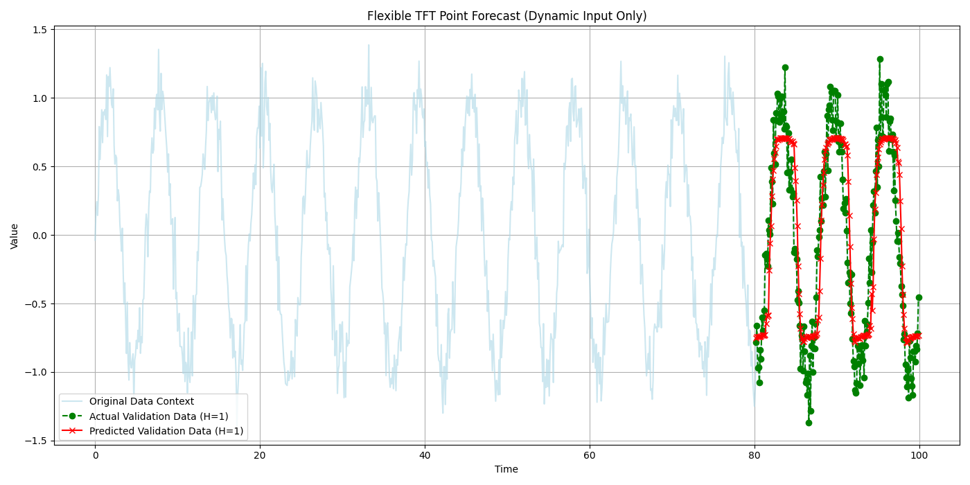
Step 1.6: Make and Visualize Quantile Predictions

Predictions will have a shape (Batch, Horizon, NumQuantiles). We visualize the median and the prediction interval.

num_samples_flex = sequences_flex.shape[0]
val_start_idx_flex = int(num_samples_flex * (1 - 0.2))
val_dynamic_inputs_flex = sequences_flex[val_start_idx_flex:]
val_actuals_flex = targets_flex[val_start_idx_flex:]

val_inputs_list_flex = [val_dynamic_inputs_flex]

print("\nMaking quantile predictions (flexible TFT)...")
val_predictions_quantiles = model_flex.predict(
    val_inputs_list_flex, verbose=0
    )
print(f"Prediction output shape: {val_predictions_quantiles.shape}")

# Visualization for one sample
sample_to_plot_flex = 0
actual_vals_flex = val_actuals_flex[sample_to_plot_flex, :, 0]
pred_quantiles_flex = val_predictions_quantiles[sample_to_plot_flex, :, :]

plot_time_axis_flex = time_flex[
    val_start_idx_flex + sequence_length_flex + sample_to_plot_flex : \
    val_start_idx_flex + sequence_length_flex + \
        sample_to_plot_flex + forecast_horizon_flex
    ]

plt.figure(figsize=(12, 6))
plt.plot(plot_time_axis_flex, actual_vals_flex,
         label='Actual Value', marker='o', linestyle='--')
plt.plot(plot_time_axis_flex, pred_quantiles_flex[:, 1], # Median (0.5)
         label='Predicted Median (q=0.5)', marker='x')
plt.fill_between(
    plot_time_axis_flex,
    pred_quantiles_flex[:, 0], # Lower quantile (q=0.1)
    pred_quantiles_flex[:, 2], # Upper quantile (q=0.9)
    color='gray', alpha=0.3,
    label='Prediction Interval (q=0.1 to q=0.9)'
)
plt.title('Flexible TFT Quantile Forecast (Dynamic Inputs Only)')
plt.xlabel('Time'); plt.ylabel('Value')
plt.legend(); plt.grid(True); plt.tight_layout()
# plt.savefig("docs/source/images/forecasting_quantile_tft_flexible.png")
plt.show()
print("Flexible TFT quantile plot generated.")

Example Output Plot (Flexible TFT):

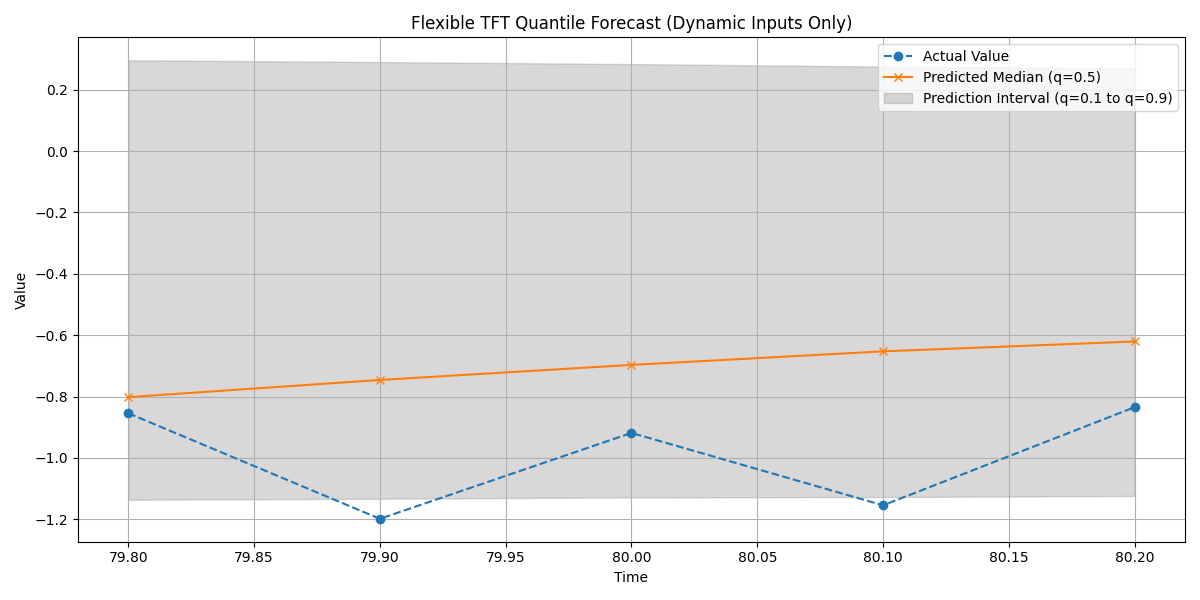
Visualization of the quantile forecast (median and interval) against actual validation data using the flexible TemporalFusionTransformer.

---

Example 2: Quantile Forecasting with Stricter TFT

This example uses the TFT class, which requires static, dynamic, and future inputs to be provided and non-None.

Workflow:

1. Generate synthetic data with static, dynamic, and future features.

2. Use reshape_xtft_data() to prepare the three separate input arrays and multi-step targets.

3. Define and compile the stricter TFT model with quantile outputs.

4. Train the model using the required three-part input list.

5. Make and visualize quantile predictions.

Step 2.1: Imports for Stricter TFT

Additional imports like StandardScaler and reshape_xtft_data.

# Imports from previous example are assumed
from sklearn.preprocessing import StandardScaler
from fusionlab.nn.transformers import TFT as TFTStricter # Alias
from fusionlab.nn.utils import reshape_xtft_data
print("\nLibraries imported for Stricter TFT Quantile Example.")

Step 2.2: Generate Synthetic Data (Multi-Feature)

We create data with distinct static, dynamic, and future features.

# define your RNG (choose any seed for reproducibility)
rng = np.random.default_rng(seed=42)
n_items_strict = 2
n_timesteps_strict = 60 # More data
date_rng_strict = pd.date_range(
    start='2020-01-01', periods=n_timesteps_strict, freq='MS'
    )
df_list_strict = []
for item_id in range(n_items_strict):
    time_idx = np.arange(n_timesteps_strict)
    value = (50 + item_id * 20 + time_idx * 0.8 +
             15 * np.sin(2 * np.pi * time_idx / 12) +
             rng.normal(0, 5, n_timesteps_strict)) # Use main rng
    static_val = item_id * 10
    future_val = (time_idx % 6 == 0).astype(float) # Event every 6 months
    item_df = pd.DataFrame({
        'Date': date_rng_strict, 'ItemID': item_id,
        'StaticFeature': static_val,
        'Month': date_rng_strict.month, # Dynamic
        'ValueLag1': pd.Series(value).shift(1), # Dynamic
        'FutureEvent': future_val, # Future
        'TargetValue': value
    })
    df_list_strict.append(item_df)
df_strict_raw = pd.concat(df_list_strict).dropna().reset_index(drop=True)
print(f"Generated data shape for stricter TFT: {df_strict_raw.shape}")

Step 2.3: Define Features & Scale

Define column roles and scale numerical features.

target_col_s = 'TargetValue'
dt_col_s = 'Date'
static_cols_s = ['ItemID', 'StaticFeature']
dynamic_cols_s = ['Month', 'ValueLag1']
future_cols_s = ['FutureEvent', 'Month'] # Month can be known future
spatial_cols_s = ['ItemID']

scaler_s = StandardScaler()
cols_to_scale_s = ['TargetValue', 'ValueLag1', 'StaticFeature']
df_strict_scaled = df_strict_raw.copy()
df_strict_scaled[cols_to_scale_s] = scaler_s.fit_transform(
    df_strict_scaled[cols_to_scale_s]
    )
print("Numerical features scaled for stricter TFT.")

Step 2.4: Prepare Sequences with reshape_xtft_data

This utility separates static, dynamic, and future features into the required arrays.

time_steps_s = 12         # 1 year lookback
forecast_horizon_s = 6    # Predict 6 months

s_data, d_data, f_data, t_data = reshape_xtft_data(
    df=df_strict_scaled, dt_col=dt_col_s, target_col=target_col_s,
    dynamic_cols=dynamic_cols_s, static_cols=static_cols_s,
    future_cols=future_cols_s, spatial_cols=spatial_cols_s,
    time_steps=time_steps_s, forecast_horizons=forecast_horizon_s,
    verbose=0
)
# Target shape for loss: (Samples, Horizon, OutputDim=1)
targets_s = t_data.astype(np.float32) # reshape_xtft_data returns (N,H,1)

print(f"\nStricter TFT - Reshaped Data Shapes:")
print(f"  Static : {s_data.shape}, Dynamic: {d_data.shape}")
print(f"  Future : {f_data.shape}, Target : {targets_s.shape}")

Step 2.5: Train/Validation Split of Sequences

Split the generated sequence arrays.

val_split_s = 0.2
n_samples_s = s_data.shape[0]
split_idx_s = int(n_samples_s * (1 - val_split_s))

X_s_train, X_s_val = s_data[:split_idx_s], s_data[split_idx_s:]
X_d_train, X_d_val = d_data[:split_idx_s], d_data[split_idx_s:]
X_f_train, X_f_val = f_data[:split_idx_s], f_data[split_idx_s:]
y_t_train, y_t_val = targets_s[:split_idx_s], targets_s[split_idx_s:]

train_inputs_s = [X_s_train, X_d_train, X_f_train]
val_inputs_s = [X_s_val, X_d_val, X_f_val]
print(f"Data split. Train sequences: {len(y_t_train)}")

Step 2.6: Define and Train Stricter TFT Model

Instantiate the stricter TFT class, providing all three input dimensions and the quantiles list.

quantiles_s = [0.1, 0.5, 0.9]
model_strict = TFTStricter( # Using the aliased stricter TFT
    static_input_dim=s_data.shape[-1],
    dynamic_input_dim=d_data.shape[-1],
    future_input_dim=f_data.shape[-1],
    forecast_horizon=forecast_horizon_s,
    quantiles=quantiles_s,
    output_dim=1, # Univariate target
    hidden_units=16, num_heads=2, num_lstm_layers=1, lstm_units=16
)
print("\nStricter TFT model for quantiles instantiated.")

loss_fn_s = combined_quantile_loss(quantiles=quantiles_s)
model_strict.compile(optimizer='adam', loss=loss_fn_s)
print("Stricter TFT compiled with quantile loss.")

print("\nStarting stricter TFT training (quantile)...")
history_s = model_strict.fit(
    train_inputs_s, # Must be [Static, Dynamic, Future]
    y_t_train,
    validation_data=(val_inputs_s, y_t_val),
    epochs=5, batch_size=16, verbose=0
)
print("Stricter TFT training finished.")
if history_s and history_s.history.get('val_loss'):
    val_loss_s = history_s.history['val_loss'][-1]
    print(f"Final validation loss (stricter TFT): {val_loss_s:.4f}")

Step 2.7: Make Predictions and Visualize (Stricter TFT)

Predictions and visualization follow a similar pattern.

print("\nMaking quantile predictions (stricter TFT)...")
val_predictions_s = model_strict.predict(val_inputs_s, verbose=0)
print(f"Prediction output shape: {val_predictions_s.shape}")

# Inverse transform (assuming 'TargetValue' was scaled by scaler_s)
# For simplicity, visualization of inverse transformed values is omitted here
# but would follow the same logic as Example 1, using scaler_s.

# Plot one sample from validation set
sample_to_plot_s = 0
actual_s = y_t_val[sample_to_plot_s, :, 0] # Scaled
pred_q_s = val_predictions_s[sample_to_plot_s, :, :] # Scaled

# Create a dummy time axis for this sample's forecast
plot_time_axis_s = np.arange(forecast_horizon_s)

plt.figure(figsize=(12, 6))
plt.plot(plot_time_axis_s, actual_s, label='Actual (Scaled)',
         marker='o', linestyle='--')
plt.plot(plot_time_axis_s, pred_q_s[:, 1], # Median
         label='Predicted Median (q=0.5, Scaled)', marker='x')
plt.fill_between(
    plot_time_axis_s, pred_q_s[:, 0], pred_q_s[:, 2],
    color='gray', alpha=0.3,
    label='Prediction Interval (q=0.1 to q=0.9, Scaled)'
)
plt.title('Stricter TFT Quantile Forecast (Validation Sample - Scaled)')
plt.xlabel('Forecast Step'); plt.ylabel('Scaled Value')
plt.legend(); plt.grid(True); plt.tight_layout()
# plt.savefig("docs/source/images/forecasting_quantile_tft_stricter.png")
plt.show()
print("Stricter TFT quantile plot generated.")

Example Output Plot (Stricter TFT - Scaled Values):

Visualization of the quantile forecast using the stricter TFT model (showing scaled values for simplicity).