Physics-Informed Transient Groundwater Flow (PiTGWFlow)

API Reference:

PiTGWFlow

The PiTGWFlow model is a powerful application of deep learning to solve a fundamental problem in hydrogeology: the 2D transient groundwater flow equation. It stands as a prime example of a Physics-Informed Neural Network (PINN), a class of models that learn directly from the governing physical laws themselves, rather than from large, labeled datasets.

Instead of traditional numerical methods like Finite Element or Finite Difference which require complex mesh generation and solve for values at discrete points, PiTGWFlow leverages a simple Multi-Layer Perceptron (MLP) as a universal function approximator. This MLP learns to represent the hydraulic head, \(h\), as a continuous and differentiable function of time \(t\) and space \((x, y)\). The model is trained not by comparing its output to known data points, but by minimizing the residual of the PDE itself at thousands of randomly sampled “collocation points” within the domain. This forces the neural network to discover a solution that is inherently consistent with the physics of groundwater flow.

Key Features

• Mesh-Free Differential Equation Solver The model uses a neural network to represent the solution space, completely bypassing the need for complex and computationally expensive mesh generation. This makes it particularly well-suited for problems with irregular or complex domain geometries.

• Unsupervised, Physics-Driven Training PiTGWFlow operates in a purely unsupervised manner. Its loss function is the Mean Squared Error of the PDE residual. In effect, the “label” it trains against is always zero—the value the PDE residual should have if the equation is perfectly satisfied. This eliminates the need for large, labeled datasets, making it ideal for data-scarce scientific applications.

• Enables Parameter Discovery (Inverse Modeling) One of the most powerful features of the PINN approach is the ability to solve inverse problems. Key physical coefficients like hydraulic conductivity (\(K\)) and specific storage (\(S_s\)) can be declared as trainable variables. The model can then infer the values of these parameters that best satisfy the governing equation, effectively discovering the underlying physics from sparse observations (when integrated into a hybrid loss).

• Simple and Familiar API Despite the complex underlying mathematics (automatic differentiation for computing PDE derivatives), the entire training process is encapsulated within the standard, user-friendly Keras workflow. The model is instantiated, compiled with .compile(), and trained with .fit(), making this advanced scientific computing technique highly accessible.

When to Use PiTGWFlow

PiTGWFlow is an excellent choice for a range of hydrogeological problems where the physics of the system are well understood.

• Solving the Forward Problem This is the classic use case for a PDE solver. When you know the physical parameters of your aquifer system (\(K\), \(S_s\), \(Q\)) and the boundary/initial conditions, you can use PiTGWFlow to accurately predict the evolution of the hydraulic head field, \(h(t, x, y)\), over any point in your domain.

• Solving the Inverse Problem This is a key strength of the PINN methodology. If you have sparse measurements of the hydraulic head at a few locations, PiTGWFlow can be used as the core of a system to infer the unknown physical parameters of the aquifer. By setting parameters like K to be learnable, the model can find the values that cause the PDE solution to best fit the sparse observations.

• For Problems Governed by Known Physics with Scarce Data The model shines in scenarios where you trust the governing equation more than you trust the availability or quality of your data. It provides a way to generate a high-fidelity, continuous solution field from the physical laws themselves, which can then be used for further analysis.

• To Obtain a Continuous and Differentiable Solution Unlike traditional numerical solvers that produce values at discrete grid points, the PiTGWFlow model learns a continuous analytical function. This is a significant advantage, as it means you can:

  1. Evaluate the solution \(h\) at any continuous coordinate \((t, x, y)\).

  2. Analytically compute its derivatives using tf.GradientTape to find other physical quantities, such as the groundwater flow velocity field (\(\mathbf{v} = -K \nabla h\)), without introducing numerical discretization errors.

The Governing Equation

The PiTGWFlow model is designed to solve one of the most fundamental equations in hydrogeology: the 2D transient groundwater flow equation. This equation is derived from Darcy’s Law and the principle of conservation of mass, and it describes how the hydraulic head (a measure of groundwater level) changes in time and space within an aquifer.

The equation is expressed as:

\[S_s \frac{\partial h}{\partial t} - K \left( \frac{\partial^2 h}{\partial x^2} + \frac{\partial^2 h}{\partial y^2} \right) - Q = 0\]

This can be written more compactly using the Laplacian operator, \(\nabla^2 h = \frac{\partial^2 h}{\partial x^2} + \frac{\partial^2 h}{\partial y^2}\), which represents the net divergence of flow at a point. The equation balances the change in storage against subsurface flow and external sources/sinks:

\[\underbrace{S_s \frac{\partial h}{\partial t}}_{\text{Change in Storage}} - \underbrace{K \nabla^2 h}_{\text{Net Subsurface Flow}} - \underbrace{Q}_{\text{Sources/Sinks}} = 0\]

Let’s break down each term:

• \(h(t, x, y)\): The hydraulic head, which is the unknown function that the neural network learns to approximate. It represents the potential energy of the groundwater at a given point and time.

• \(\frac{\partial h}{\partial t}\) (The Transient Term): This is the rate of change of the hydraulic head over time. It quantifies how quickly water levels are rising or falling. A positive value means the water level is increasing, and vice-versa.

• \(\nabla^2 h\) (The Laplacian Term): This term describes the net “curvature” of the hydraulic head surface in space. A non-zero Laplacian indicates an imbalance of flow. For instance, at the center of a pumping well’s cone of depression, the Laplacian is large and negative, indicating that water is flowing into that point from all directions faster than it is flowing out.

• \(S_s\) (Specific Storage): A crucial physical property of the aquifer. It represents the volume of water that a unit volume of the aquifer releases from storage for every unit decline in hydraulic head, due to the compressibility of both the water and the aquifer’s porous skeleton.

• \(K\) (Hydraulic Conductivity): A parameter that measures how easily water can move through the soil or rock. High-permeability materials like sand have a high \(K\), while low-permeability materials like clay have a very low \(K\).

• \(Q\) (Source/Sink Term): This term accounts for any water being artificially added to (e.g., via injection wells) or removed from (e.g., via pumping wells) the aquifer system per unit volume.

Architectural Workflow: A Deep Dive

The PiTGWFlow architecture is elegant in its simplicity. It combines a standard neural network with a custom, physics-driven training loop that enforces the governing equation described above.

1. The Neural Network Surrogate

The core of the model is a simple Multi-Layer Perceptron (MLP). In the context of PINNs, this MLP acts as a universal function approximator. Its job is to learn a continuous function, \(h_{NN}(\theta; t, x, y)\), that serves as a surrogate for the true, unknown solution \(h\).

The inputs to this network are only the continuous spatio-temporal coordinates, and its output is a single scalar value—the predicted hydraulic head at that point.

\[h_{NN} = \text{MLP}(\theta; [t, x, y])\]

Here, \(\theta\) represents all the trainable weights and biases of the MLP.

2. The Physics-Informed Training Step

This is where the “physics” is injected. Instead of comparing the network’s output to ground-truth labels, the training process forces the network’s output to obey the PDE. This happens in several stages within the custom train_step:

• A. Collocation Point Sampling: For each training step, the model receives a batch of random spatio-temporal points, \((t, x, y)\), called collocation points. These points are sampled from within the problem’s domain and are where the physical law will be evaluated and enforced.

• B. Forward Pass: The coordinates of these collocation points are fed through the MLP surrogate to get the predicted head values, \(h_{NN}\), at each of those points.

• C. Automatic Differentiation: This is the core mechanism of PINNs. The model uses TensorFlow’s GradientTape, a powerful tool that acts like a “computational microscope,” to calculate the exact partial derivatives of the MLP’s output (\(h_{NN}\)) with respect to its inputs (\(t, x, y\)). It computes all terms needed for the PDE:

  \[\frac{\partial h_{NN}}{\partial t}, \quad \frac{\partial h_{NN}}{\partial x}, \quad \frac{\partial h_{NN}}{\partial y}, \quad \frac{\partial^2 h_{NN}}{\partial x^2}, \quad \frac{\partial^2 h_{NN}}{\partial y^2}\]

• D. Residual Calculation: These analytically computed derivatives are then plugged into the governing groundwater flow equation to calculate the PDE residual, \(R\), for each collocation point. A perfect solution would have \(R=0\) everywhere.

  \[R = S_s \frac{\partial h_{NN}}{\partial t} - K \left( \frac{\partial^2 h_{NN}}{\partial x^2} + \frac{\partial^2 h_{NN}}{\partial y^2} \right) - Q\]

• E. Loss Computation: The model’s loss function, \(\mathcal{L}\), is simply the Mean Squared Error of these residuals. The goal of training is to find the network weights \(\theta\) (and any learnable physical parameters) that make this loss as close to zero as possible.

  \[\mathcal{L}(\theta, K, S_s, Q) = \frac{1}{N}\sum_{i=1}^{N} (R_i)^2\]

3. End-to-End Optimization

The final step is to compute the gradient of the physics loss \(\mathcal{L}\) with respect to all trainable variables in the model. This includes:

1. The weights and biases of the MLP surrogate (\(\theta\)).

2. Any physical parameters that were defined as Learnable (e.g., LearnableK, LearnableSs).

The optimizer (e.g., Adam) then uses these gradients to update all variables, simultaneously tuning the neural network to better approximate the solution field and tuning the physical parameters to values that best describe the system.

Complete Example

This example demonstrates a complete workflow for using PiTGWFlow to solve a forward problem where we also ask the model to perform parameter discovery for the hydraulic conductivity (\(K\)).

Step 1: Imports and Setup

First, we import the necessary libraries from TensorFlow and fusionlab-learn, and set up a directory to save our results.

import os
import numpy as np
import tensorflow as tf
import matplotlib.pyplot as plt

# FusionLab imports
from fusionlab.nn.pinn import PiTGWFlow
from fusionlab.params import LearnableK

os.environ['TF_CPP_MIN_LOG_LEVEL'] = '3' # Suppress logs

EXERCISE_OUTPUT_DIR = "./pitgwflow_outputs"
os.makedirs(EXERCISE_OUTPUT_DIR, exist_ok=True)

Step 2: Generate Collocation Points

Unlike traditional models, PINNs are not trained on labeled data. Instead, they learn by minimizing the PDE residual at thousands of randomly sampled points, known as collocation points, within the problem’s spatio-temporal domain.

We also create a dummy_y tensor of zeros. This is required to satisfy the Keras .fit() API, which expects data in an (X, y) format, but these dummy targets are completely ignored during training. The actual loss is derived solely from the physics.

# Configuration
N_POINTS = 5000
BATCH_SIZE = 128

# Generate random (t, x, y) coordinates within a defined domain
tf.random.set_seed(42)
coords = {
    "t": tf.random.uniform((N_POINTS, 1), 0, 10), # Time from 0 to 10
    "x": tf.random.uniform((N_POINTS, 1), -1, 1), # x from -1 to 1
    "y": tf.random.uniform((N_POINTS, 1), -1, 1), # y from -1 to 1
}

# Dummy targets are required for the Keras API but are ignored
dummy_y = tf.zeros((N_POINTS, 1))

# Create an efficient tf.data.Dataset for training
dataset = tf.data.Dataset.from_tensor_slices(
    (coords, dummy_y)
).shuffle(N_POINTS).batch(BATCH_SIZE).prefetch(tf.data.AUTOTUNE)

print(f"Generated {N_POINTS} collocation points for training.")

Step 3: Define, Compile, and Train PiTGWFlow

We now instantiate the PiTGWFlow model. Note how we pass Ss and Q as fixed Python floats, but we pass K as a LearnableK object. This tells the model to treat \(K\) as a trainable parameter to be discovered during optimization.

Because the model uses its own internal PDE residual loss, we only need to call .compile() to set up the optimizer.

# Instantiate PiTGWFlow with a learnable K
pinn_model = PiTGWFlow(
    hidden_units=[40, 40, 40],
    activation='tanh',
    K=LearnableK(1.0), # The model will infer this value
    Ss=1e-4,           # Fixed value
    Q=0.0              # Fixed value
)

# Compile the model (loss is handled internally)
pinn_model.compile(optimizer=tf.keras.optimizers.Adam(learning_rate=1e-3))

print("Training PiTGWFlow model...")
history = pinn_model.fit(
    dataset,
    epochs=25, # Use more epochs for a more converged solution
    verbose=0
)
print("Training complete.")

# Extract the final learned value for K
# The name 'param_K' is set internally by the model
learned_k = [v for v in pinn_model.trainable_variables if 'param_K' in v.name]
if learned_k:
    # The model learns log(K), so we take the exp()
    final_k_value = tf.exp(learned_k[0]).numpy().mean()
    print(f"Final Learned K: {final_k_value.mean():.4f}")

Step 4: Visualize Training History

After training, we should always inspect the learning curve. A steadily decreasing pde_loss indicates that the neural network is successfully learning a function that minimizes the PDE residual, thus satisfying the governing physical law.

from fusionlab.nn.models.utils import plot_history_in

print("\nPlotting training history...")
plot_history_in(history, metrics={"PDE Loss": ["pde_loss"]})

Expected Output Plot:

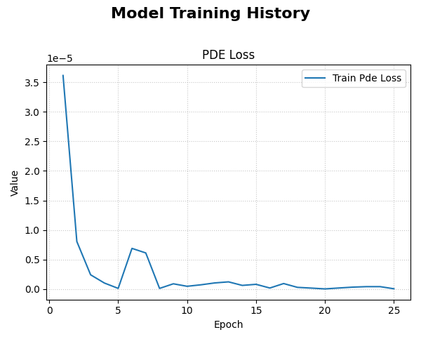
An example plot showing the PDE loss decreasing over epochs. The logarithmic scale helps visualize the rapid reduction in error as the model learns to satisfy the physics.

Step 5: Visualize the Learned Solution

The key advantage of the PINN is that it has learned a continuous function \(h(t, x, y)\). We can now evaluate this function on a regular grid of points to visualize the full solution field at a specific moment in time.

# 1. Create a meshgrid for visualization at a specific time slice
t_slice = 5.0
x_range = np.linspace(-1, 1, 100)
y_range = np.linspace(-1, 1, 100)
X, Y = np.meshgrid(x_range, y_range)

# 2. Prepare grid coordinates for prediction
x_flat = tf.convert_to_tensor(X.ravel(), dtype=tf.float32)
y_flat = tf.convert_to_tensor(Y.ravel(), dtype=tf.float32)
t_flat = tf.fill(x_flat.shape, t_slice)

grid_coords = {
    't': tf.reshape(t_flat, (-1, 1)),
    'x': tf.reshape(x_flat, (-1, 1)),
    'y': tf.reshape(y_flat, (-1, 1))
}

# 3. Predict the hydraulic head 'h' on the grid
h_pred_flat = pinn_model.predict(grid_coords)
h_pred_grid = tf.reshape(h_pred_flat, X.shape)

# 4. Plot the contour of the solution
plt.figure(figsize=(9, 7))
contour = plt.contourf(X, Y, h_pred_grid, 100, cmap='jet_r')
plt.colorbar(contour, label='Hydraulic Head (h)')
plt.title(f'Learned Hydraulic Head Solution at t = {t_slice}')
plt.xlabel('x-coordinate')
plt.ylabel('y-coordinate')
plt.axis('equal')
plt.show()

Expected Output Plot:

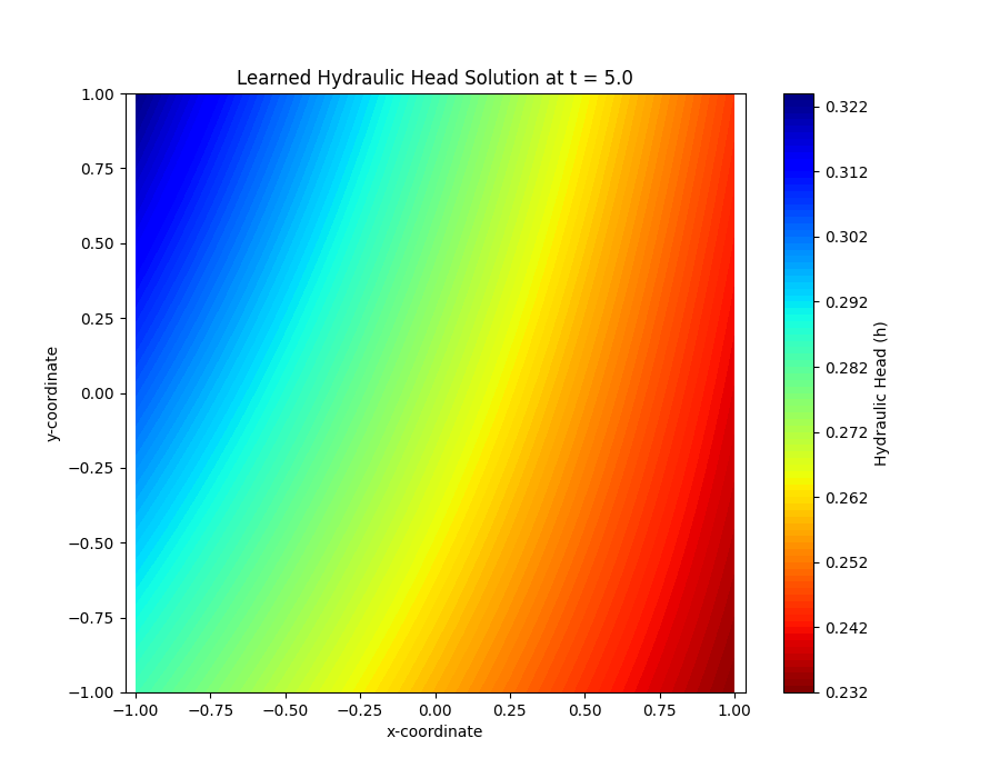
A 2D contour map showing the continuous hydraulic head field learned by the model. The smooth contours demonstrate the differentiable nature of the neural network solution.

Next Steps

Note

Now that you understand the theory and the complete workflow for PiTGWFlow, you can apply these concepts to solve your own forward or inverse hydrogeological problems.

Proceed to the exercises for more hands-on practice: Exercise: Solving a Forward Problem with PiTGWFlow