Exercise: Anomaly Detection

Welcome to this exercise on anomaly detection using fusionlab-learn! In this guide, you’ll walk through practical examples of using the specialized anomaly detection components available in the fusionlab.nn.anomaly_detection module. These components can help you build models to identify unusual patterns in your time series data.

Learning Objectives:

• Understand and implement an LSTM Autoencoder for reconstruction-based anomaly detection.

• Learn the conceptual use of the SequenceAnomalyScoreLayer for feature-based scoring within larger models.

• Apply the PredictionErrorAnomalyScore layer to derive anomaly scores from model prediction errors.

Let’s get started!

Prerequisites

Before you begin, ensure you have fusionlab-learn and its common dependencies installed. For visualizations, matplotlib is also needed.

pip install fusionlab-learn matplotlib scikit-learn

Exercise 1: Unsupervised Anomaly Detection with LSTM Autoencoder

In this first exercise, we’ll build and train an LSTM Autoencoder. The core idea is that an autoencoder trained on “normal” data will struggle to reconstruct anomalous data points or sequences, leading to higher reconstruction errors for those anomalies.

Workflow:

1. Generate synthetic time series data with some manually injected anomalies.

2. Preprocess the data: scale it and create input sequences.

3. Define, compile, and train the LSTMAutoencoderAnomaly model.

4. Use the trained model to reconstruct the sequences and calculate reconstruction errors.

5. Identify anomalies by setting a threshold on these errors.

6. Visualize the original data, detected anomalies, and the error scores.

Step 1.1: Imports and Setup

First, let’s import all the necessary libraries.

import numpy as np
import pandas as pd
import tensorflow as tf
import matplotlib.pyplot as plt
from sklearn.preprocessing import StandardScaler
import warnings
import os

# FusionLab imports
from fusionlab.nn.anomaly_detection import LSTMAutoencoderAnomaly
from fusionlab.nn.utils import create_sequences # For sequence prep

# Suppress warnings and TF logs for cleaner output
warnings.filterwarnings('ignore')
tf.get_logger().setLevel('ERROR')
if hasattr(tf, 'autograph'): # Check for autograph availability
    tf.autograph.set_verbosity(0)

# Directory for saving any output images from this exercise
exercise_output_dir = "./anomaly_detection_exercise_outputs"
os.makedirs(exercise_output_dir, exist_ok=True)

print("Libraries imported for LSTM Autoencoder exercise.")

Step 1.2: Generate Synthetic Data with Anomalies

We’ll create a simple sine wave and add some obvious anomalies to it.

np.random.seed(42) # For reproducibility
time_points = np.arange(0, 200, 0.5)
# Base normal signal
normal_signal = np.sin(time_points * 0.5) + \
                np.random.normal(0, 0.1, len(time_points))
# Inject some anomalies
data_with_anomalies = normal_signal.copy()
data_with_anomalies[50:60] += 2.0  # A positive spike/shift
data_with_anomalies[150:155] -= 1.5 # A negative dip/shift

df_exercise = pd.DataFrame({
    'Time': time_points,
    'Value': data_with_anomalies
    })
print("Generated data shape for exercise:", df_exercise.shape)

# Let's visualize our data
plt.figure(figsize=(12, 3))
plt.plot(df_exercise['Time'], df_exercise['Value'],
         label='Data with Injected Anomalies')
plt.title("Synthetic Time Series for Anomaly Detection Exercise")
plt.xlabel("Time Index")
plt.ylabel("Value")
plt.legend()
plt.grid(True)
# To save for documentation:
# plt.savefig(os.path.join(
#    exercise_output_dir, "exercise_ad_synthetic_data.png"))
plt.show()

Expected Plot 1.2:

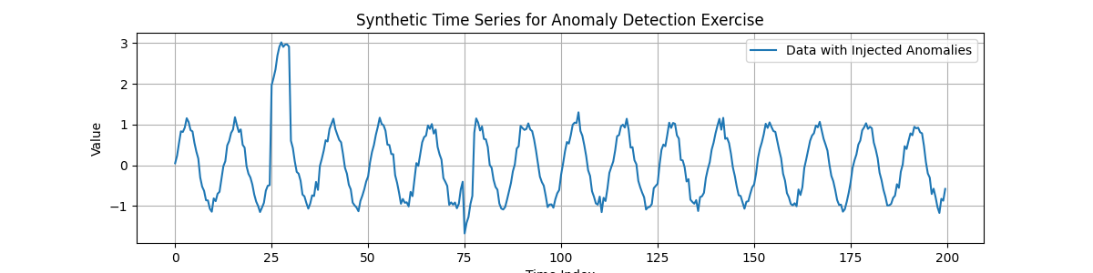
Synthetic time series with manually injected anomalous periods.

Step 1.3: Preprocessing - Scaling and Sequence Creation

Neural networks generally perform better with scaled data. We’ll use StandardScaler. Then, we’ll create overlapping sequences from our time series, as LSTMs operate on sequences. For an autoencoder, the input sequence is also its own target for reconstruction.

scaler_ad_ex = StandardScaler()
df_exercise['Value_Scaled'] = scaler_ad_ex.fit_transform(
    df_exercise[['Value']]
    )
print("\nData scaled using StandardScaler.")

sequence_len_ex = 20 # Length of sequences for the autoencoder

# Using create_sequences: target_col is 'Value_Scaled',
# forecast_horizon=0 means reconstruct the input sequence itself.
sequences_ex, _ = create_sequences(
    df_exercise[['Value_Scaled']],
    sequence_length=sequence_len_ex,
    target_col='Value_Scaled',
    forecast_horizon=0, # Reconstruct the input sequence
    drop_last=False,    # Keep all possible sequences
    verbose=0
)
# For autoencoder, input (X) and target (y) are the same
X_train_ae = sequences_ex.reshape(
    sequences_ex.shape[0], sequence_len_ex, 1 # Features=1
    ).astype(np.float32)
y_train_ae = X_train_ae.copy() # Target is the input itself

print(f"Created sequences for autoencoder. X_train shape: "
      f"{X_train_ae.shape}")

Expected Output 1.3:

Data scaled using StandardScaler.
Created sequences for autoencoder. X_train shape: (381, 20, 1)

Step 1.4: Define LSTM Autoencoder Model

Now, we instantiate our LSTMAutoencoderAnomaly. Key parameters are latent_dim (size of the compressed representation) and lstm_units. n_features should match our input, and n_repeats should match sequence_len_ex for reconstruction.

latent_dim_ae = 8
lstm_units_ae = 16 # Units in LSTM layers

lstm_ae_model_ex = LSTMAutoencoderAnomaly(
    latent_dim=latent_dim_ae,
    lstm_units=lstm_units_ae,
    n_features=X_train_ae.shape[-1], # Should be 1
    n_repeats=sequence_len_ex,     # Output sequence length
    num_encoder_layers=1,
    num_decoder_layers=1,
    activation='linear' # Good for reconstructing potentially unbounded scaled data
)
print("\nLSTM Autoencoder model defined.")

Step 1.5: Compile and Train the Autoencoder

We compile with ‘adam’ optimizer and ‘mse’ loss, then train the model. The model learns to reconstruct the input sequences.

lstm_ae_model_ex.compile(optimizer='adam', loss='mse')
print("Autoencoder compiled. Starting training...")

# Build the model with input shape before fitting
lstm_ae_model_ex.build(input_shape=(None, sequence_len_ex, X_train_ae.shape[-1]))
# lstm_ae_model_ex.summary() # Optional: view model structure

history_ae = lstm_ae_model_ex.fit(
    X_train_ae, y_train_ae, # Input and target are the same
    epochs=20,        # Train for more epochs for better learning
    batch_size=16,
    shuffle=True,     # Shuffle sequences during training
    verbose=0         # Suppress Keras fit logs for this example
)
print("Training finished.")
if history_ae and history_ae.history.get('loss'):
    print(f"Final training loss (MSE): {history_ae.history['loss'][-1]:.4f}")

Expected Output 1.5:

(The loss value will vary slightly due to random initialization)

Autoencoder compiled. Starting training...
Training finished.
Final training loss (MSE): 0.0617

Step 1.6: Calculate Reconstruction Errors (Anomaly Scores)

After training, we use the model to reconstruct all sequences and calculate the Mean Squared Error (MSE) for each. This MSE serves as our anomaly score for each sequence window.

print("\nCalculating reconstruction errors...")
reconstruction_errors_ex = lstm_ae_model_ex.compute_reconstruction_error(
    X_train_ae # Pass all sequences to get their errors
).numpy() # Get as NumPy array
print(f"Reconstruction errors shape: {reconstruction_errors_ex.shape}")

# Map sequence errors back to original time points for plotting
# (Assign error of a sequence to its last point for simplicity)
errors_mapped_ex = np.full(len(df_exercise), np.nan)
for i in range(len(reconstruction_errors_ex)):
    # Ensure index is within bounds
    end_point_idx = i + sequence_len_ex - 1
    if end_point_idx < len(errors_mapped_ex):
        errors_mapped_ex[end_point_idx] = reconstruction_errors_ex[i]

df_exercise['ReconstructionError'] = errors_mapped_ex

Expected Output 1.6:

Calculating reconstruction errors...
Reconstruction errors shape: (381,)

Step 1.7: Detect Anomalies using a Threshold

We define a threshold based on the distribution of reconstruction errors (e.g., the 95th percentile). Sequences with errors above this threshold are flagged as anomalies.

# Define threshold (e.g., based on error distribution percentile)
# Ensure to use only non-NaN errors for percentile calculation
valid_errors_ex = df_exercise['ReconstructionError'].dropna()
if not valid_errors_ex.empty:
    threshold_ex = np.percentile(valid_errors_ex, 95)
    df_exercise['Is_Anomaly'] = df_exercise['ReconstructionError'] > threshold_ex
    print(f"\nAnomaly threshold (95th percentile error): {threshold_ex:.4f}")
    print(f"Number of points flagged as anomalies: {df_exercise['Is_Anomaly'].sum()}")
else:
    print("\nNo valid reconstruction errors to calculate threshold.")
    df_exercise['Is_Anomaly'] = False # Default if no errors

Expected Output 1.7:

(Values will vary)

Anomaly threshold (95th percentile error): 0.3643
Number of points flagged as anomalies: 19

Step 1.8: Visualize Results

Finally, plot the original data with detected anomalies and the reconstruction error over time.

fig_ae, ax_ae = plt.subplots(2, 1, figsize=(14, 8), sharex=True)

ax_ae[0].plot(df_exercise['Time'], df_exercise['Value'],
              label='Original Data', zorder=1)
anomalies_ex = df_exercise[df_exercise['Is_Anomaly']]
if not anomalies_ex.empty:
    ax_ae[0].scatter(anomalies_ex['Time'], anomalies_ex['Value'],
                     color='red', label='Detected Anomaly',
                     zorder=5, s=50)
ax_ae[0].set_ylabel('Value')
ax_ae[0].set_title('Time Series with Detected Anomalies (LSTM Autoencoder)')
ax_ae[0].legend(); ax_ae[0].grid(True)

ax_ae[1].plot(df_exercise['Time'], df_exercise['ReconstructionError'],
              label='Reconstruction Error (MSE per Sequence)',
              color='orange')
if 'threshold_ex' in locals() and np.isfinite(threshold_ex):
    ax_ae[1].axhline(threshold_ex, color='red', linestyle='--',
                     label=f'Threshold ({threshold_ex:.2f})')
ax_ae[1].set_ylabel('Reconstruction Error (MSE)')
ax_ae[1].set_xlabel('Time')
ax_ae[1].set_title('Reconstruction Error and Anomaly Threshold')
ax_ae[1].legend(); ax_ae[1].grid(True)

plt.tight_layout()
# To save for documentation:
# plt.savefig(os.path.join(
#    exercise_output_dir, "exercise_ad_lstm_ae_results.png"))
plt.show()

Expected Plot 1.8:

Top: Original signal with detected anomalies highlighted. Bottom: Reconstruction error over time with the anomaly threshold.

Discussion of Exercise 1:

The LSTM Autoencoder learns the “normal” patterns in the time series. When it encounters sequences that are significantly different (our injected anomalies), it cannot reconstruct them well, leading to a spike in the reconstruction error. By setting a threshold on this error, we can flag these anomalous periods. The choice of sequence_length, latent_dim, lstm_units, and the error threshold are important hyperparameters that would typically be tuned.

---

Exercise 2: Using SequenceAnomalyScoreLayer (Conceptual)

The SequenceAnomalyScoreLayer is a component, not a standalone model. It’s designed to be part of a larger neural network (like XTFT). It takes learned features from preceding layers and passes them through a small Multi-Layer Perceptron (MLP) to output a single anomaly score per input sample.

Concept: Imagine you have a model that processes time series and extracts meaningful features (e.g., the output of an LSTM encoder or an attention mechanism). You can then feed these features into the SequenceAnomalyScoreLayer to get an anomaly score. This score can then be used in a custom loss function to train the entire model in an anomaly-aware manner.

Step 2.1: Imports and Setup

We only need TensorFlow and the layer itself.

import tensorflow as tf
from fusionlab.nn.anomaly_detection import SequenceAnomalyScoreLayer
print("\nLibraries imported for SequenceAnomalyScoreLayer exercise.")

Step 2.2: Instantiate and Use the Layer

Let’s simulate some “learned features” and see how the layer processes them.

# Assume 'learned_features_ex2' is the output of a preceding layer
# Shape: (Batch, FeatureDim)
batch_size_ex2 = 16
feature_dim_ex2 = 64 # Example dimension of learned features
learned_features_ex2 = tf.random.normal(
    (batch_size_ex2, feature_dim_ex2), dtype=tf.float32
    )

# Instantiate the scoring layer
anomaly_scorer_ex2 = SequenceAnomalyScoreLayer(
    hidden_units=[32, 16], # Define MLP structure within the layer
    activation='relu',
    dropout_rate=0.1,
    final_activation='linear' # Output an unbounded score
)

# Pass features through the layer to get scores
# In a real model, this happens within its 'call' method.
anomaly_scores_ex2 = anomaly_scorer_ex2(
    learned_features_ex2, training=False # Set training appropriately
    )

print(f"\nInput features shape for scorer: {learned_features_ex2.shape}")
print(f"Output anomaly scores shape: {anomaly_scores_ex2.shape}")
print("Sample scores:", anomaly_scores_ex2.numpy()[:5].flatten())

Expected Output 2.2:

Input features shape for scorer: (16, 64)
Output anomaly scores shape: (16, 1)
Sample scores: [ 0.19996917 -0.8162031   0.6714213  -0.36490577  1.3606443 ]

Discussion of Exercise 2:

This layer provides a trainable mechanism to derive anomaly scores from abstract feature representations. To make it useful, it needs to be part of an end-to-end model trained with a loss function that relates these scores to actual anomalies or desired behavior (e.g., penalizing high scores for normal data if labels are available, or using it in an unsupervised reconstruction + anomaly score setup). Refer to the XTFT ‘feature_based’ strategy in the User Guide for more on integration.

---

Exercise 3: Using PredictionErrorAnomalyScore

The PredictionErrorAnomalyScore layer directly calculates an anomaly score based on the discrepancy (error) between true values (y_true) and a model’s predicted values (y_pred) for a sequence.

Concept: If a forecasting model makes large errors for a particular sequence, that sequence might be anomalous or represent a regime the model hasn’t learned well. This layer quantifies that prediction error.

Step 3.1: Imports and Setup

We need TensorFlow and the layer.

import tensorflow as tf
import numpy as np # For a more visible error injection
from fusionlab.nn.anomaly_detection import PredictionErrorAnomalyScore
print("\nLibraries imported for PredictionErrorAnomalyScore exercise.")

Step 3.2: Instantiate and Use the Layer

We’ll create dummy y_true and y_pred tensors, then see how the layer calculates scores.

# Configuration for dummy data
batch_size_ex3 = 4
time_steps_ex3 = 10
features_ex3 = 1 # Univariate example

# Dummy true values
y_true_ex3 = tf.random.normal(
    (batch_size_ex3, time_steps_ex3, features_ex3), dtype=tf.float32
    )
# Dummy predicted values with some errors
y_pred_ex3_np = y_true_ex3.numpy() + np.random.normal(
    scale=0.5, size=y_true_ex3.shape
    ).astype(np.float32)
# Inject a larger error into one sample's prediction
y_pred_ex3_np[1, 3, 0] += 4.0 # Large error for sample 1, time step 3
y_pred_ex3 = tf.constant(y_pred_ex3_np)

# --- Instantiate with MAE and Mean Aggregation ---
error_scorer_mean_ex3 = PredictionErrorAnomalyScore(
    error_metric='mae',     # Use Mean Absolute Error
    aggregation='mean'    # Average errors across time steps
)
anomaly_scores_mean_ex3 = error_scorer_mean_ex3([y_true_ex3, y_pred_ex3])

# --- Instantiate with MAE and Max Aggregation ---
error_scorer_max_ex3 = PredictionErrorAnomalyScore(
    error_metric='mae',
    aggregation='max'     # Take max error across time steps
)
anomaly_scores_max_ex3 = error_scorer_max_ex3([y_true_ex3, y_pred_ex3])

print(f"\nInput y_true shape: {y_true_ex3.shape}")
print(f"Input y_pred shape: {y_pred_ex3.shape}")
print("\n--- MAE + Mean Aggregation ---")
print(f"Output anomaly scores shape: {anomaly_scores_mean_ex3.shape}")
print(f"Example Scores (Mean Error per sequence): \n"
      f"{anomaly_scores_mean_ex3.numpy().flatten()}")
print("\n--- MAE + Max Aggregation ---")
print(f"Output anomaly scores shape: {anomaly_scores_max_ex3.shape}")
print(f"Example Scores (Max Error per sequence): \n"
      f"{anomaly_scores_max_ex3.numpy().flatten()}")

Expected Output 3.2:

(Error values will vary. Note how the score for the second sequence (index 1) is likely higher with ‘max’ aggregation due to the injected large error.)

Input y_true shape: (4, 10, 1)
Input y_pred shape: (4, 10, 1)

--- MAE + Mean Aggregation ---
Output anomaly scores shape: (4, 1)
Example Scores (Mean Error per sequence):
[0.25818387 0.83212453 0.5759385  0.52767694]

--- MAE + Max Aggregation ---
Output anomaly scores shape: (4, 1)
Example Scores (Max Error per sequence):
[0.7972139 4.6388383 1.0303739 1.0196161]

Discussion of Exercise 3:

The PredictionErrorAnomalyScore layer provides a straightforward way to quantify how “surprising” a sequence is to a pre-trained forecasting model. These scores can be directly used in a loss function to penalize the main forecasting model when it makes large errors, effectively making it anomaly-aware. This aligns with the ‘prediction_based’ anomaly detection strategy in XTFT.