HALNet (Hybrid Attentive LSTM Network)
- API Reference:
The Hybrid Attentive LSTM Network (HALNet) is a powerful,
data-driven model designed for complex, multi-horizon time series
forecasting. It forms the architectural core of the
PIHALNet model but is provided
as a standalone tool for general-purpose forecasting tasks that do
not require physics-informed constraints.
HALNet leverages a sophisticated encoder-decoder framework,
integrating multi-scale LSTMs and a suite of advanced attention
mechanisms to capture complex temporal patterns from static, dynamic
past, and known future inputs.
Key Features
Flexible Encoder-Decoder Architecture: The model can operate in two distinct modes via the
modeparameter:pihal_like: A standard sequence-to-sequence architecture where the encoder processes past data and the decoder uses future data.
`tft_like`: An architecture inspired by the Temporal Fusion Transformer where known future inputs are used to enrich both the historical context (encoder) and the future context (decoder).
Encoder-Decoder Architecture: Correctly processes historical data (in the encoder) and future context (in the decoder) separately, making it robust to differing lookback and forecast horizon lengths.
Advanced Input Handling: Accepts three distinct types of inputs: static, dynamic (past observed), and known future features. It can optionally use
VariableSelectionNetwork(VSN) for intelligent, learnable feature selection and embedding for each input type.Multi-Scale Temporal Processing: Employs a
MultiScaleLSTMin the encoder to capture temporal dependencies at various user-defined resolutions (via thescalesparameter).Rich Attention Mechanisms: Uses a suite of attention layers to effectively fuse information from different sources:
CrossAttentionallows the decoder to focus on the most relevant parts of the encoded historical context.HierarchicalAttentionandMemoryAugmentedAttentionfurther refine the decoder’s context.MultiResolutionAttentionFusionintegrates the final set of features before prediction.
Probabilistic Forecasting: Employs
QuantileDistributionModelingto output forecasts for specifiedquantiles, enabling the estimation of prediction uncertainty. It produces standard point forecasts ifquantilesisNone.
When to Use HALNet
HALNet is an excellent choice for complex forecasting problems
where:
You have rich inputs, including static metadata, historical time series, and information about the future.
The underlying temporal dynamics are complex and may exist at multiple time scales.
You need to forecast multiple time steps into the future (multi-horizon forecasting).
Capturing long-range dependencies and complex interactions between different features is important for accuracy.
Architectural Workflow
HALNet’s architecture is organized into an encoder-decoder
structure. The key difference between its operational modes lies in
how it handles the future_input tensor.
Input Modes: tft_like vs. pihal_like
mode='pihal_like'(Standard Encoder-Decoder):In this mode,
future_inputis expected to have a time dimension equal to theforecast_horizon.Encoder: Processes only the dynamic_input (of length \(T_{past}\)) to create a summary of the past.
Decoder: Uses the encoder’s summary along with the static_input and the entire future_input to generate the forecast. This is a clean and robust separation of concerns.
mode='tft_like'(TFT-Style Inputs):This mode requires the
future_inputtensor to span both the lookback and forecast periods, with a time dimension of \(T_{past} + T_{future}\).Encoder: The future_input is sliced. Its historical part (length \(T_{past}\)) is concatenated with the dynamic_input and fed into the encoder. This provides the encoder with richer context about past events.
Decoder: The future part of the future_input (length \(T_{future}\)) is used as context for generating the prediction.
Subsequent Steps (Common to Both Modes):
Initial Feature Processing:
Both static and time-varying inputs (dynamic and future) are first processed to create feature representations. If
use_vsnisTrue, each input type is passed through its ownVariableSelectionNetworkand a subsequentGatedResidualNetwork(GRN). IfFalse, they are processed by standardDenselayers.Encoder Path:
The encoder’s role is to create a rich, contextualized summary of all past information.
The historical parts of the dynamic_input and future_input (a slice of length \(T_{past}\)) are combined.
This combined tensor is passed through a
MultiScaleLSTM.The outputs from different LSTM scales are aggregated by
aggregate_multiscale()into a single 3D tensor, \(\mathbf{E} \in \mathbb{R}^{B \times T' \times D_{enc}}\), which represents the complete encoded history. \(T'\) is the (potentially sliced) time dimension of the past.
Decoder Path:
The decoder prepares the context for the forecast window (\(T_{future}\) or
forecast_horizon).The static context vector is tiled across the forecast horizon.
The future part of the future_input tensor (of length \(T_{future}\)) is combined with the tiled static context.
This combined tensor is projected by a
Denselayer to create the initial decoder context, \(\mathbf{D}_{init} \in \mathbb{R}^{B \times T_{future} \times D_{attn}}\).
Attention-Based Fusion:
The decoder context acts as a query to the encoder’s output sequences (which serve as keys and values) via
CrossAttention. This allows the model to focus on the most relevant historical information for each future time step it predicts. This is where the model intelligently combines the past and future.Cross-Attention: The decoder context \(\mathbf{D}_{init}\) acts as the query to attend to the encoded history \(\mathbf{E}\) (which serves as the key and value).
\[\mathbf{A}_{cross} = \text{CrossAttention}(\mathbf{D}_{init}, \mathbf{E})\]Context Refinement: The output of the cross-attention is further processed through residual connections, normalization, and other self-attention layers (HierarchicalAttention, MemoryAugmentedAttention, MultiResolutionAttentionFusion) to build a highly refined feature representation for the forecast period.
Residual Connection: The output of the cross-attention is added to the initial decoder input and normalized, a standard technique for stabilizing deep models.
\[\mathbf{D}' = \text{LayerNorm}(\mathbf{D}_{init} + \text{GRN}(\mathbf{A}_{cross}))\]Self-Attention: Further attention layers (Hierarchical, Memory, Multi-Resolution Fusion) refine this fused context \(\mathbf{D}'\) through self-attention mechanisms.
Final Aggregation and Output:
The final feature tensor from the attention blocks, which has a shape of \((B, T_{future}, D_{feat})\), is aggregated along the time dimension using the specified
final_aggstrategy (e.g., taking the ‘last’ step or ‘average’). This produces a single vector per sample.This vector is passed to the
MultiDecoderto generate predictions for each step in the horizon.Finally,
QuantileDistributionModelingmaps the decoder’s output to the final point or quantile forecasts.
Complete Example
This example demonstrates a complete workflow for HALNet using the
tft_like mode, which has the more complex data requirement.
Step 1: Imports and Setup
First, we import all necessary libraries and set up the environment.
 1import os
 2import numpy as np
 3import pandas as pd
 4import tensorflow as tf
 5import matplotlib.pyplot as plt
 6from sklearn.preprocessing import StandardScaler, LabelEncoder
 7import warnings
 8
 9# FusionLab imports
10from fusionlab.nn.models import HALNet
11from fusionlab.nn.utils import reshape_xtft_data
12from fusionlab.nn.models.utils import plot_history_in
13from fusionlab._fusionlog import fusionlog
14
15logger = fusionlog().get_fusionlab_logger(__name__)
16warnings.filterwarnings('ignore')
17tf.get_logger().setLevel('ERROR')
18
19EXERCISE_OUTPUT_DIR = "./halnet_exercise_outputs"
20os.makedirs(EXERCISE_OUTPUT_DIR, exist_ok=True)
Step 2: Generate and Prepare Synthetic Data
We generate a synthetic dataset and use reshape_xtft_data to create the three required input arrays (static, dynamic, future).
 1# Configuration
 2N_ITEMS = 3
 3N_TIMESTEPS_PER_ITEM = 100
 4TIME_STEPS = 14
 5FORECAST_HORIZON = 7
 6TARGET_COL = 'Value'
 7DT_COL = 'Date'
 8
 9# Generate synthetic data (code omitted for brevity, see exercise page)
10# ...
11# Preprocessing (LabelEncoding, Scaling)
12# ...
13
14# For this example, we'll create dummy arrays with the correct shapes
15# that `reshape_xtft_data` would output.
16n_sequences = N_ITEMS * (N_TIMESTEPS_PER_ITEM - TIME_STEPS - FORECAST_HORIZON + 1)
17
18static_data = np.random.rand(n_sequences, 2)  # e.g., ItemID, Category
19dynamic_data = np.random.rand(n_sequences, TIME_STEPS, 3) # e.g., ValueLag1, DayOfWeek
20# Future data spans both past and future windows for 'tft_like' mode
21future_data = np.random.rand(n_sequences, TIME_STEPS + FORECAST_HORIZON, 2)
22targets = np.random.rand(n_sequences, FORECAST_HORIZON, 1)
23
24print(f"Generated data shapes for 'tft_like' mode:")
25print(f"  Static:  {static_data.shape}")
26print(f"  Dynamic: {dynamic_data.shape}")
27print(f"  Future:  {future_data.shape}")
28print(f"  Target:  {targets.shape}")
Step 3: Define, Compile, and Train HALNet
We instantiate the model, specifying mode=’tft_like’, and then compile and train it.
 1# Split data into training and validation sets
 2train_inputs = [arr[:-20] for arr in [static_data, dynamic_data, future_data]]
 3val_inputs = [arr[-20:] for arr in [static_data, dynamic_data, future_data]]
 4train_targets, val_targets = targets[:-20], targets[-20:]
 5
 6# Instantiate HALNet for 'tft_like' operation
 7halnet_model = HALNet(
 8    static_input_dim=static_data.shape[-1],
 9    dynamic_input_dim=dynamic_data.shape[-1],
10    future_input_dim=future_data.shape[-1],
11    output_dim=1,
12    forecast_horizon=FORECAST_HORIZON,
13    max_window_size=TIME_STEPS,
14    mode='tft_like', # Specify the mode
15    use_vsn=False,
16    hidden_units=16,
17    attention_units=16
18)
19
20# Compile and train
21halnet_model.compile(optimizer='adam', loss='mse', metrics=['mae'])
22print("\\nTraining HALNet model...")
23history = halnet_model.fit(
24    train_inputs,
25    train_targets,
26    validation_data=(val_inputs, val_targets),
27    epochs=10,
28    batch_size=32,
29    verbose=0 # Set to 1 to see progress
30)
31print("Training complete.")
Step 4: Visualize Training History
Use the plot_history_in utility to visualize the loss curves.
1print("\\nPlotting training history...")
2plot_history_in(
3    history,
4    metrics={"Loss": ["loss"], "MAE": ["mae"]},
5    layout='subplots',
6    title="HALNet Training and Validation History"
7)
Example Output Plot:
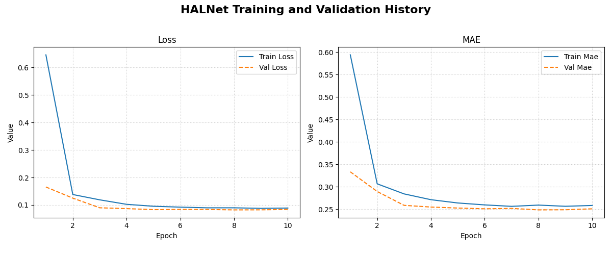
An example plot showing the training and validation loss and Mean Absolute Error (MAE) over epochs. This helps in diagnosing model fit and convergence.