XTFT Forecasting with Anomaly Detection

This example demonstrates how to leverage the anomaly detection features integrated within the XTFT model. Incorporating anomaly information during training can potentially make the model more robust to irregularities and improve forecasting performance, especially on noisy real-world data.

We will adapt the setup from the Advanced Forecasting with XTFT example and show two main approaches for integrating anomaly detection into a multi-step quantile forecasting task:

1. Strategy 1: Using Pre-computed Anomaly Scores: We’ll first calculate anomaly scores externally (e.g., using compute_anomaly_scores()) and then incorporate them into the training loss using a combined loss function (combined_total_loss()).

2. Strategy 2: Using Prediction-Based Errors: We’ll configure XTFT to use the anomaly_detection_strategy = 'prediction_based', where the anomaly signal is derived directly from prediction errors during training via a specialized loss function (prediction_based_loss()).

Prerequisites

Ensure you have fusionlab-learn and its dependencies installed:

pip install fusionlab-learn matplotlib scikit-learn joblib

Strategy 1: Using Pre-computed Anomaly Scores

In this strategy, we assume we have a way to generate anomaly scores for our target variable before training the main forecasting model. These scores are then used to create a combined loss function.

Step 1.1: Imports and Setup

Import standard libraries and fusionlab components.

import numpy as np
import pandas as pd
import tensorflow as tf
import matplotlib.pyplot as plt
from sklearn.model_selection import train_test_split
from sklearn.preprocessing import StandardScaler
import os
import joblib

# FusionLab imports
from fusionlab.nn.transformers import XTFT
from fusionlab.nn.utils import (
    reshape_xtft_data,
    compute_anomaly_scores # For pre-calculating scores
)
from fusionlab.nn.losses import (
    combined_quantile_loss,
    combined_total_loss,    # For Strategy 1
    prediction_based_loss   # For Strategy 2
)
from fusionlab.nn.components import AnomalyLoss # For combined_total_loss

# Suppress warnings and TF logs
import warnings
warnings.filterwarnings('ignore')
tf.get_logger().setLevel('ERROR')
if hasattr(tf, 'autograph'):
    tf.autograph.set_verbosity(0)

output_dir_xtft_anom = "./xtft_anomaly_example_output"
os.makedirs(output_dir_xtft_anom, exist_ok=True)
print("Libraries imported for XTFT Anomaly Detection Example.")

Step 1.2: Generate Synthetic Data (with Anomalies)

We create multi-item time series data, similar to the advanced XTFT example, but intentionally inject some anomalies (spikes/dips) into the ‘Sales’ target variable for one of the items.

n_items = 3
n_timesteps = 48 # More data for anomaly context
rng_seed = 123
np.random.seed(rng_seed)

date_rng = pd.date_range(
    start='2019-01-01', periods=n_timesteps, freq='MS')
df_list = []

for item_id in range(n_items):
    time_idx = np.arange(n_timesteps)
    sales = (
        100 + item_id * 30 + time_idx * (1.5 + item_id * 0.3) +
        25 * np.sin(2 * np.pi * time_idx / 12) + # Yearly seasonality
        np.random.normal(0, 8, n_timesteps)  # Base noise
    )
    # Inject anomalies for item_id 1
    if item_id == 1:
        sales[10] = sales[10] + 80 # Positive spike
        sales[25] = sales[25] - 60 # Negative dip
        print(f"Injected anomalies for ItemID {item_id} at indices 10 and 25.")

    temp = (15 + 10 * np.sin(2 * np.pi * (time_idx % 12) / 12 + np.pi) +
            np.random.normal(0, 1.5, n_timesteps))
    promo = np.random.randint(0, 2, n_timesteps)

    item_df = pd.DataFrame({
        'Date': date_rng, 'ItemID': f'item_{item_id}',
        'Month': date_rng.month, 'Temperature': temp,
        'PlannedPromotion': promo, 'Sales': sales
    })
    item_df['PrevMonthSales'] = item_df['Sales'].shift(1)
    df_list.append(item_df)

df_raw_anom = pd.concat(df_list).dropna().reset_index(drop=True)
print(f"\nGenerated data with anomalies, shape: {df_raw_anom.shape}")

Step 1.3: Define Features & Scale

Define column roles and scale the numerical features.

target_col_anom = 'Sales'
dt_col_anom = 'Date'
static_cols_anom = ['ItemID']
dynamic_cols_anom = ['Month', 'Temperature', 'PrevMonthSales']
future_cols_anom = ['PlannedPromotion', 'Month']
spatial_cols_anom = ['ItemID'] # For grouping
scalers_anom = {}
num_cols_to_scale_anom = ['Temperature', 'PrevMonthSales', 'Sales']
df_scaled_anom = df_raw_anom.copy()

for col in num_cols_to_scale_anom:
    if col in df_scaled_anom.columns:
        scaler = StandardScaler()
        df_scaled_anom[col] = scaler.fit_transform(df_scaled_anom[[col]])
        scalers_anom[col] = scaler
        print(f"Scaled column: {col}")

scalers_path_anom = os.path.join(output_dir_xtft_anom, "xtft_anom_scalers.joblib")
joblib.dump(scalers_anom, scalers_path_anom)
print(f"Scalers saved to {scalers_path_anom}")

Step 1.4: Prepare Sequences

Use reshape_xtft_data to create sequence arrays.

time_steps_anom = 12
forecast_horizons_anom = 6
static_cols_for_reshape = [] # No additional static features here

s_data, d_data, f_data, t_data = reshape_xtft_data(
    df=df_scaled_anom, dt_col=dt_col_anom, target_col=target_col_anom,
    dynamic_cols=dynamic_cols_anom, static_cols=static_cols_for_reshape,
    future_cols=future_cols_anom, spatial_cols=spatial_cols_anom,
    time_steps=time_steps_anom, forecast_horizons=forecast_horizons_anom,
    verbose=0
)
print(f"\nSequence shapes: S={s_data.shape if s_data is not None else 'None'}, "
      f"D={d_data.shape}, F={f_data.shape}, T={t_data.shape}")

Step 1.5: Pre-compute Anomaly Scores

Calculate anomaly scores for the target sequences.

print("\nCalculating anomaly scores for target sequences...")
anomaly_scores_all_seq = compute_anomaly_scores(
    y_true=t_data, method='statistical', verbose=0
)
print(f"Computed anomaly scores shape: {anomaly_scores_all_seq.shape}")

Step 1.6: Train/Validation Split (Including Anomaly Scores)

Split all arrays: static, dynamic, future, target, and anomaly scores.

val_split_frac_anom = 0.2
n_seq_anom = t_data.shape[0]
split_idx_anom = int(n_seq_anom * (1 - val_split_frac_anom))

X_s_train, X_s_val = (s_data[:split_idx_anom], s_data[split_idx_anom:]) \
    if s_data is not None else (None, None)
X_d_train, X_d_val = d_data[:split_idx_anom], d_data[split_idx_anom:]
X_f_train, X_f_val = f_data[:split_idx_anom], f_data[split_idx_anom:]
y_train, y_val = t_data[:split_idx_anom], t_data[split_idx_anom:]

anomaly_scores_train = anomaly_scores_all_seq[:split_idx_anom]
anomaly_scores_val = anomaly_scores_all_seq[split_idx_anom:]

train_inputs = [X_s_train, X_d_train, X_f_train]
val_inputs = [X_s_val, X_d_val, X_f_val]
print("\nData (including anomaly scores) split into Train/Validation.")

Step 1.7: Define XTFT Model and Combined Loss (Strategy 1)

Instantiate XTFT. Use combined_total_loss with an AnomalyLoss component and the pre-computed anomaly_scores_train.

quantiles_anom = [0.1, 0.5, 0.9]
anomaly_loss_weight_s1 = 0.1 # Weight for Strategy 1

s_dim_anom = X_s_train.shape[-1] if X_s_train is not None else 0
d_dim_anom = X_d_train.shape[-1]
f_dim_anom = X_f_train.shape[-1] if X_f_train is not None else 0

model_s1 = XTFT(
    static_input_dim=s_dim_anom, dynamic_input_dim=d_dim_anom,
    future_input_dim=f_dim_anom,
    forecast_horizon=forecast_horizons_anom,
    quantiles=quantiles_anom, output_dim=1,
    hidden_units=16, embed_dim=8, num_heads=2,
    lstm_units=16, attention_units=16, max_window_size=time_steps_anom,
    anomaly_loss_weight=anomaly_loss_weight_s1 # Passed to AnomalyLoss
)

anomaly_loss_component_s1 = AnomalyLoss(weight=anomaly_loss_weight_s1)
loss_s1 = combined_total_loss(
    quantiles=quantiles_anom,
    anomaly_layer=anomaly_loss_component_s1,
    anomaly_scores=tf.constant(anomaly_scores_train, dtype=tf.float32)
)
model_s1.compile(
    optimizer=tf.keras.optimizers.Adam(learning_rate=0.005),
    loss=loss_s1
)
print("\nXTFT (Strategy 1) compiled with combined loss.")

Step 1.8: Train Model (Strategy 1)

Train the model.

print("Starting XTFT training (Strategy 1: Pre-computed Scores)...")
history_s1 = model_s1.fit(
    train_inputs, y_train,
    validation_data=(val_inputs, y_val),
    epochs=5, batch_size=16, verbose=1
)
print("Training (Strategy 1) finished.")
if history_s1 and history_s1.history.get('val_loss'):
    print(f"S1 - Final validation loss: {history_s1.history['val_loss'][-1]:.4f}")

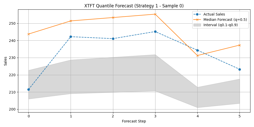
Step 1.9: Prediction & Visualization (Strategy 1)

Prediction and visualization are standard.

print("\nMaking predictions with Strategy 1 model...")
predictions_scaled_s1 = model_s1.predict(val_inputs, verbose=0)

# Inverse Transform
target_scaler_s1 = scalers_anom.get(target_col_anom)
if target_scaler_s1:
    num_val_s1 = val_inputs[0].shape[0] if val_inputs[0] is not None else val_inputs[1].shape[0]
    num_q_s1 = len(quantiles_anom)
    output_dim_s1 = 1 # Assuming univariate target

    pred_reshaped_s1 = predictions_scaled_s1.reshape(-1, num_q_s1 * output_dim_s1)
    predictions_inv_s1 = target_scaler_s1.inverse_transform(pred_reshaped_s1)
    predictions_final_s1 = predictions_inv_s1.reshape(
        num_val_s1, forecast_horizons_anom, num_q_s1
    )
    y_val_reshaped_s1 = y_val.reshape(-1, output_dim_s1)
    y_val_inv_s1 = target_scaler_s1.inverse_transform(y_val_reshaped_s1)
    y_val_final_s1 = y_val_inv_s1.reshape(
        num_val_s1, forecast_horizons_anom, output_dim_s1
    )
    print("Predictions and actuals inverse transformed for Strategy 1.")
else:
    print("Warning: Target scaler not found for Strategy 1. Plotting scaled values.")
    predictions_final_s1 = predictions_scaled_s1
    y_val_final_s1 = y_val

# Visualize for one sample
sample_to_plot_s1 = 0
actual_vals_s1 = y_val_final_s1[sample_to_plot_s1, :, 0]
pred_quantiles_s1 = predictions_final_s1[sample_to_plot_s1, :, :]
time_axis_s1 = np.arange(forecast_horizons_anom)

plt.figure(figsize=(10, 5))
plt.plot(time_axis_s1, actual_vals_s1, label='Actual Sales', marker='o', linestyle='--')
plt.plot(time_axis_s1, pred_quantiles_s1[:, 1], label='Median Forecast (q=0.5)', marker='x')
plt.fill_between(
    time_axis_s1, pred_quantiles_s1[:, 0], pred_quantiles_s1[:, 2],
    color='gray', alpha=0.3, label='Interval (q0.1-q0.9)'
)
plt.title(f'XTFT Quantile Forecast (Strategy 1 - Sample {sample_to_plot_s1})')
plt.xlabel('Forecast Step'); plt.ylabel('Sales')
plt.legend(); plt.grid(True); plt.tight_layout()
# plt.savefig(os.path.join(output_dir_xtft_anom, "s1_forecast_plot.png"))
plt.show()
print("Strategy 1: Plot generated.")

# [out] Training (Strategy 1) finished.
# S1 - Final validation loss: 0.4350

Example Output Plot:

---

Strategy 2: Using Prediction-Based Errors

This approach configures XTFT to derive anomaly signals directly from its own prediction errors during training.

(Data from Steps 1.2 (df_raw_anom), 1.3 (df_scaled_anom, scalers_anom), 1.4 (s_data, d_data, f_data, t_data), and 1.6 (train_inputs, val_inputs, y_train, y_val) are assumed to be available here. We do not use the pre-computed `anomaly_scores_all_seq` for this strategy.)

Step 2.1: Define XTFT Model (Prediction-Based)

Instantiate XTFT with anomaly_detection_strategy=’prediction_based’ and provide anomaly_loss_weight.

print("\n--- Configuring for Strategy 2: 'prediction_based' ---")
anomaly_weight_s2 = 0.05 # Weight for prediction error penalty

# Re-use dimensions from Strategy 1 data prep for consistency
s_dim_s2 = X_s_train.shape[-1] if X_s_train is not None else 0

model_s2 = XTFT(
    static_input_dim=s_dim_s2,
    dynamic_input_dim=X_d_train.shape[-1],
    future_input_dim=X_f_train.shape[-1] if X_f_train is not None else 0,
    forecast_horizon=forecast_horizons_anom,
    quantiles=quantiles_anom, output_dim=1,
    hidden_units=16, embed_dim=8, num_heads=2,
    lstm_units=16, attention_units=16, max_window_size=time_steps_anom,
    anomaly_detection_strategy='prediction_based',
    anomaly_loss_weight=anomaly_weight_s2
)
print("XTFT (Strategy 2) instantiated with 'prediction_based'.")

Step 2.2: Compile with Prediction-Based Loss

Use the prediction_based_loss() factory.

loss_s2 = prediction_based_loss(
    quantiles=quantiles_anom,
    anomaly_loss_weight=anomaly_weight_s2
)
model_s2.compile(
    optimizer=tf.keras.optimizers.Adam(learning_rate=0.005),
    loss=loss_s2
)
print("XTFT (Strategy 2) compiled with prediction_based_loss.")

Step 2.3: Train Model (Strategy 2)

Train the model. The combined loss is handled internally.

print("\nStarting XTFT training (Strategy 2: Prediction-Based)...")
history_s2 = model_s2.fit(
    train_inputs, y_train,
    validation_data=(val_inputs, y_val),
    epochs=5, batch_size=16, verbose=1
)
print("Training (Strategy 2) finished.")
if history_s2 and history_s2.history.get('val_loss'):
    print(f"S2 - Final validation loss: {history_s2.history['val_loss'][-1]:.4f}")

Step 2.4: Prediction & Visualization (Strategy 2)

The prediction and visualization process is identical to Strategy 1, using model_s2.

print("\nMaking predictions with Strategy 2 model...")
predictions_scaled_s2 = model_s2.predict(val_inputs, verbose=0)
print(f"Prediction output shape (Strategy 2): {predictions_scaled_s2.shape}")

# --- Inverse Transform (Example) ---
target_scaler_s2 = scalers_anom.get(target_col_anom)
if target_scaler_s2:
    num_val_s2 = val_inputs[0].shape[0] if val_inputs[0] is not None \
        else val_inputs[1].shape[0]
    num_q_s2 = len(quantiles_anom)
    output_dim_s2 = 1 # Assuming univariate

    pred_reshaped_s2 = predictions_scaled_s2.reshape(-1, num_q_s2 * output_dim_s2)
    if output_dim_s2 == 1: # Common case
        predictions_inv_s2 = target_scaler_s2.inverse_transform(pred_reshaped_s2)
        predictions_final_s2 = predictions_inv_s2.reshape(
            num_val_s2, forecast_horizons_anom, num_q_s2
        )
        # y_val was already inverse transformed for Strategy 1 if target_scaler_s1 existed
        # Assuming y_val_final_s1 is available from Strategy 1 for comparison
        # If not, inverse transform y_val here using target_scaler_s2
        y_val_final_s2 = y_val_final_s1 # Re-use if scaler is the same
        print("Predictions inverse transformed for Strategy 2.")
    else:
        print("Inverse transform for multi-output quantiles for S2 not shown.")
        predictions_final_s2 = predictions_scaled_s2
        y_val_final_s2 = y_val # Plot scaled if multi-output inverse is complex
else:
    print("Warning: Target scaler not found for Strategy 2. Plotting scaled values.")
    predictions_final_s2 = predictions_scaled_s2
    y_val_final_s2 = y_val # Plot scaled

# --- Visualization (Example for one sample) ---
if predictions_final_s2 is not None and y_val_final_s2 is not None:
    sample_to_plot_s2 = 0
    actual_vals_s2 = y_val_final_s2[sample_to_plot_s2, :, 0]
    pred_quantiles_s2 = predictions_final_s2[sample_to_plot_s2, :, :]
    time_axis_s2 = np.arange(forecast_horizons_anom)

    plt.figure(figsize=(10, 5))
    plt.plot(time_axis_s2, actual_vals_s2, label='Actual Sales', marker='o', linestyle='--')
    plt.plot(time_axis_s2, pred_quantiles_s2[:, 1], label='Median Forecast (q=0.5)', marker='x')
    plt.fill_between(
        time_axis_s2, pred_quantiles_s2[:, 0], pred_quantiles_s2[:, 2],
        color='orange', alpha=0.3, label='Interval (q0.1-q0.9) - Strategy 2'
    )
    plt.title(f'XTFT Quantile Forecast (Strategy 2 - Sample {sample_to_plot_s2})')
    plt.xlabel('Forecast Step'); plt.ylabel('Sales')
    plt.legend(); plt.grid(True); plt.tight_layout()
    # plt.savefig(os.path.join(output_dir_xtft_anom, "s2_forecast_plot.png"))
    plt.show()
    print("Strategy 2: Plot generated.")
else:
    print("Strategy 2: Skipping plot due to missing prediction/actual data.")

 # [Out] Training (Strategy 2) finished.
 # S2 - Final validation loss: 0.7625

Example Output Plot (Conceptual):

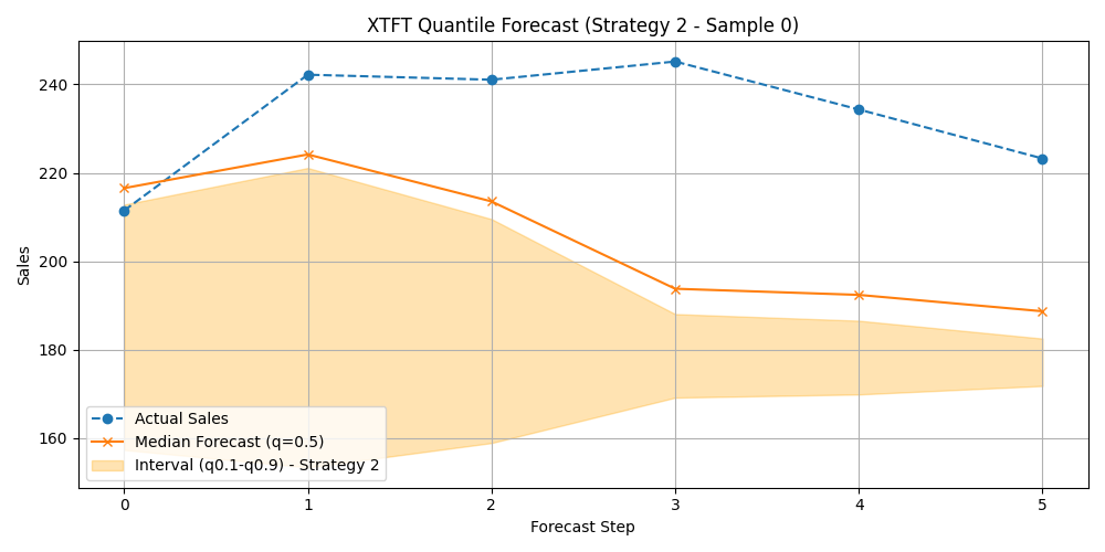
Conceptual visualization of XTFT quantile forecast where training incorporated an anomaly detection strategy.