Spatial Data Utilities

The fusionlab.utils.spatial_utils module provides a collection of specialized functions for common data processing and analysis tasks involving geospatial data (e.g., longitude/latitude coordinates).

This guide covers the primary utilities for spatial clustering, stratified sampling, coordinate-based filtering and merging, and other data manipulation techniques essential for preparing data for spatiotemporal models.

---

Spatial Clustering (create_spatial_clusters)

API Reference:

create_spatial_clusters()

Spatial clustering is a fundamental technique in exploratory data analysis used to identify natural groupings or “regions” within a set of geographic points. This can be invaluable for tasks like defining study areas, creating regional features for a model, or understanding the spatial structure of your data.

The create_spatial_clusters function provides a high-level, convenient interface for applying popular clustering algorithms from scikit-learn directly to the coordinate data in your DataFrame.

Supported Algorithms

The function acts as a wrapper for three distinct algorithms, each suited for different scenarios:

• KMeans (`algorithm=’kmeans’`): This is a partitioning algorithm that aims to divide data points into a pre-defined number of clusters (\(k\)). It works by minimizing the within-cluster sum of squares. It is fast and effective for finding well-separated, spherical-shaped clusters.

• DBSCAN (`algorithm=’dbscan’`): A density-based algorithm that groups together points that are closely packed, marking as outliers points that lie alone in low-density regions. It is excellent for discovering clusters of arbitrary shape and does not require the number of clusters to be specified beforehand. Its behavior is controlled by the eps (neighborhood distance) and min_samples parameters.

• Agglomerative Clustering (`algorithm=’agglo’`): A hierarchical clustering method that starts with each data point as its own cluster and iteratively merges the closest pairs of clusters until the desired number of clusters is reached. It is useful for understanding nested structures in the data.

Key Features

• Multiple Algorithms: Easily switch between KMeans, DBSCAN, and Agglomerative clustering via the algorithm parameter.

• Automatic `k` Detection: For KMeans, if you do not specify n_clusters, the function can automatically estimate the optimal number of clusters using silhouette and elbow analysis.

• Automatic Coordinate Scaling: Clustering algorithms are sensitive to feature scales. With auto_scale=True (the default), the function automatically standardizes your coordinate data before clustering to ensure distances are weighted equally.

• Integrated Visualization: Setting view=True provides immediate visual feedback by generating a scatter plot of the data points, colored by their newly assigned cluster labels.

Usage Example 1: KMeans with a Fixed Number of Clusters

This example shows the most straightforward use case, where we have two clear groups of points and we ask KMeans to find them.

import pandas as pd
import numpy as np
from fusionlab.utils.spatial_utils import create_spatial_clusters

# 1. Create a sample DataFrame with two clear groups of points
np.random.seed(42)
group1 = np.random.rand(20, 2) * 2
group2 = (np.random.rand(20, 2) * 2) + 5
df = pd.DataFrame(np.vstack([group1, group2]), columns=['lon', 'lat'])

# 2. Use KMeans to find 2 spatial clusters and visualize them
df_clustered = create_spatial_clusters(
    df=df,
    spatial_cols=['lon', 'lat'],
    algorithm="kmeans",
    n_clusters=2, # Manually set to 2 for this example
    view=True,
    cluster_col='my_regions' # Custom name for the cluster column
)

# 3. Display the head of the resulting DataFrame
print("\nDataFrame with new cluster column:")
print(df_clustered.head())

Expected Output:

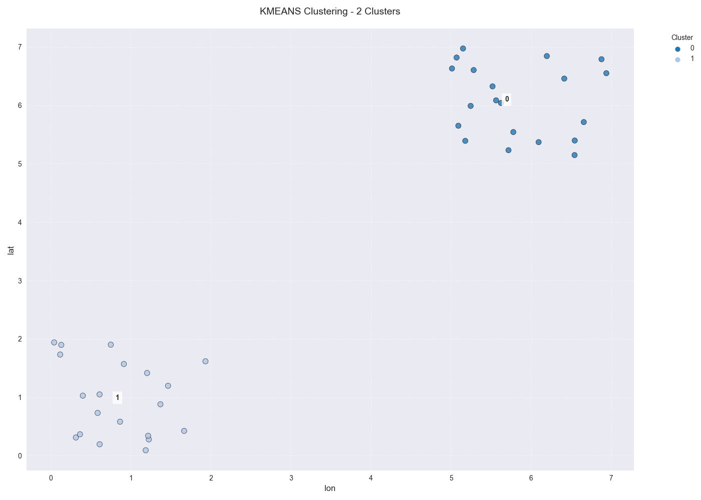
A scatter plot showing the data points colored by their two assigned KMeans cluster labels.

DataFrame with new cluster column:
       lon       lat  my_regions
0  0.749080  1.901429           0
1  1.463988  1.536165           0
2  1.458941  1.054942           0
3  1.238539  1.171827           0
4  0.413864  0.763176           0

Usage Example 2: DBSCAN with Custom Parameters

This example demonstrates how to use a different algorithm (DBSCAN) and pass algorithm-specific parameters (like eps and min_samples) through the **kwargs.

# Use the same DataFrame 'df' from the previous example

# Use DBSCAN to find density-based clusters
df_dbscan = create_spatial_clusters(
    df=df,
    spatial_cols=['lon', 'lat'],
    algorithm="dbscan",
    view=False, # Disable plot for this example
    # Pass DBSCAN-specific parameters via kwargs
    eps=0.5,
    min_samples=3
)

# Display the new cluster labels
print("\nCluster labels assigned by DBSCAN:")
print(df_dbscan['region'].value_counts())

Expected Output:

Cluster labels assigned by DBSCAN:
region
0    20
1    20
Name: count, dtype: int64

---

Stratified Spatial Sampling

Working with large geospatial datasets presents a unique challenge: how do you create a smaller, representative subset for training or analysis? A simple random sample is often insufficient, as it may miss or under-represent important spatial patterns and rare categories.

Stratified sampling is the solution. It works by dividing the entire dataset into homogeneous subgroups, or “strata,” and then drawing a proportional number of samples from each one. This ensures that the final sample is a faithful microcosm of the original data’s spatial and categorical distribution.

The utilities in fusionlab-learn implement a sophisticated stratification strategy that combines two methods:

1. Spatial Binning: The geographic area is first divided into a grid based on the coordinate columns (e.g., longitude and latitude). This is done using quantile-based bins, which ensures that each spatial “tile” contains a similar number of data points, effectively stratifying by location.

2. Categorical Stratification: The spatial bins are then further subdivided by any categorical columns provided in the stratify_by parameter (e.g., year, geology_type).

By sampling from these highly specific strata (e.g., “points in the northwest quadrant that are in the ‘Sedimentary’ category from the year 2020”), the resulting subset is exceptionally representative.

Core Sampling Functions

The library provides two functions for this task, each with a specific purpose.

spatial_sampling

API Reference:

spatial_sampling()

This is the fundamental function for drawing a single, representative sample from a large dataset. It is the ideal tool for creating a holdout test set or a smaller dataset for exploratory analysis that accurately reflects the characteristics of the full dataset.

batch_spatial_sampling

API Reference:

batch_spatial_sampling()

This utility extends spatial_sampling by dividing the total desired sample into multiple, non-overlapping batches. This is extremely useful for:

• Training models on datasets that are too large to fit into memory at once.

• Creating stratified folds for a robust cross-validation scheme.

Usage Example 1: Creating a Single Stratified Sample

This example shows how to use spatial_sampling to draw a single 5% sample from a dataset, stratified by location and category.

import pandas as pd
import numpy as np
from fusionlab.utils.spatial_utils import spatial_sampling

# 1. Create a large dummy DataFrame
np.random.seed(42)
df_large = pd.DataFrame({
    "longitude": np.random.uniform(-120, -80, 10000),
    "latitude": np.random.uniform(30, 50, 10000),
    "category": np.random.choice(['A', 'B', 'C'], 10000, p=[0.6, 0.3, 0.1])
})

# 2. Draw a single 5% sample, stratified by space and category
sampled_df = spatial_sampling(
    data=df_large,
    sample_size=0.05, # 5% of total data
    stratify_by=['category'],
    spatial_bins=5,
    verbose=1
)

# 3. Print the shape and category distribution of the sample
print(f"\nShape of single stratified sample: {sampled_df.shape}")
print("\nOriginal category distribution (%):")
print(df_large['category'].value_counts(normalize=True) * 100)
print("\nSampled category distribution (%):")
print(sampled_df['category'].value_counts(normalize=True) * 100)

Expected Output:

Shape of single stratified sample: (500, 3)

Original category distribution (%):
category
A    60.41
B    29.53
C    10.06
Name: proportion, dtype: float64

Sampled category distribution (%):
category
A    60.4
B    29.6
C    10.0
Name: proportion, dtype: float64

Usage Example 2: Creating Multiple Batches

This example uses batch_spatial_sampling to achieve the same total sample size (10%) but splits it into 5 non-overlapping batches.

from fusionlab.utils.spatial_utils import batch_spatial_sampling

# Use the same df_large from the previous example

# 2. Draw a total sample of 10% of the data, split into 5 batches
batches = batch_spatial_sampling(
    data=df_large,
    sample_size=0.1, # 10% of total data
    n_batches=5,
    stratify_by=['category'],
    spatial_bins=5,
    verbose=1
)

# 3. Print the shape of each generated batch
print("\n--- Shape of Generated Batches ---")
for i, batch in enumerate(batches):
    print(f"Batch {i+1}: {batch.shape}")

Expected Output:

Creating 5 stratified batches with a total of 1,000 samples...
Batch Sampling Progress: 100%|...| 5/5 [00:00<00:00, ...]
Batch sampling completed. 5 batches created.

--- Shape of Generated Batches ---
Batch 1: (200, 3)
Batch 2: (200, 3)
Batch 3: (200, 3)
Batch 4: (200, 3)
Batch 5: (200, 3)

---

Filtering and Merging by Position

These utilities are designed to select or combine data based on spatial proximity, which is a common requirement when working with real-world geospatial datasets that may not have perfectly aligned coordinates.

filter_position

API Reference:

filter_position()

This function acts like a “spatial query” tool. Its primary purpose is to select rows from a DataFrame that correspond to a specific geographic point of interest. It offers two powerful modes for matching:

• Exact Matching (`find_closest=False`): This mode is useful when you need to retrieve data for a known, precise location, such as a specific monitoring well or sensor with exact coordinates.

• Approximate Matching (`find_closest=True`): This is the more advanced feature. It is designed for situations where an exact coordinate match might not exist in your dataset. It finds the data point that is numerically closest to your target coordinate, as long as it falls within a given threshold distance. This is ideal for querying gridded data or aligning with points from a different source.

Usage Example

import pandas as pd
from fusionlab.utils.spatial_utils import filter_position

# 1. Create a sample DataFrame of sensor locations
df = pd.DataFrame({
    'lon': [10.0, 10.05, 12.5],
    'lat': [20.0, 20.06, 22.0],
    'value': [100, 110, 120]
})

# 2. Example of an exact match
# This will only find the row where lon is exactly 12.5
df_exact = filter_position(
    df, pos=12.5, pos_cols='lon', find_closest=False
)
print("--- Exact Match Result ---")
print(df_exact)

# 3. Example of an approximate match
# Find points "near" (10.01, 20.01) within a 0.1 degree radius
df_approx = filter_position(
    df,
    pos=(10.01, 20.01),
    pos_cols=('lon', 'lat'),
    find_closest=True,
    threshold=0.1
)
print("\n--- Approximate Match Result ---")
print(df_approx)

Expected Output:

--- Exact Match Result ---
   lon    lat  value
2  12.5   22.0    120

--- Approximate Match Result ---
   lon    lat  value
0  10.00  20.00    100
1  10.05  20.06    110

dual_merge

API Reference:

dual_merge()

Think of this function as a “spatially-aware” pandas.merge. It is designed to solve the common problem of joining two DataFrames that should represent the same locations but have slightly different, misaligned coordinates (e.g., due to different data sources, precision, or map projections).

Instead of requiring an exact match on coordinate columns, it can join rows based on spatial proximity, finding the nearest point in the second DataFrame for each point in the first.

Usage Example

from fusionlab.utils.spatial_utils import dual_merge

# 1. Create two DataFrames with slightly misaligned coordinates
df1_wells = pd.DataFrame({
    'well_id': ['W1', 'W2'],
    'longitude': [10.01, 12.52],
    'latitude': [20.02, 22.03],
})
df2_geology = pd.DataFrame({
    'lon': [10.0, 12.5],
    'lat': [20.0, 22.0],
    'rock_type': ['Sandstone', 'Shale']
})

# 2. Merge them by finding the closest spatial points
df_merged = dual_merge(
    df1_wells, df2_geology,
    feature_cols=('longitude', 'latitude'), # df1 uses these names
    find_closest=True,
    threshold=0.1 # Max distance to consider a match
)
print(df_merged)

Expected Output:

  well_id  longitude  latitude  lon   lat  rock_type
0      W1      10.01     20.02  10.0  20.0  Sandstone
1      W2      12.52     22.03  12.5  22.0      Shale

---

Other Utilities

Extracting Data Zones (extract_zones_from)

API Reference:

extract_zones_from()

This is a powerful data exploration and filtering tool. Its purpose is to isolate subsets of your data—or “zones”—based on a value criterion. For example, you can use it to “find all locations where subsidence is greater than 50mm” or “show me the data points corresponding to the top 10% of rainfall events.” The threshold=’auto’ feature, which uses percentiles, makes this kind of exploratory analysis particularly easy.

Usage Example

from fusionlab.utils.spatial_utils import extract_zones_from

# 1. Create sample data
data = {'value': np.arange(1, 101)}
df_zones = pd.DataFrame(data)

# 2. Extract the zone containing the top 5% of values
top_5_percent_zone = extract_zones_from(
    z=df_zones['value'],
    threshold='auto',
    percentile=95, # The threshold will be the 95th percentile
    condition='above'
)
print(top_5_percent_zone)

Expected Output:

   value
0     96
1     97
2     98
3     99
4    100

Coordinate Column Extraction (extract_coordinates)

API Reference:

extract_coordinates()

This is a convenience utility designed to reduce boilerplate code. It robustly finds and extracts common coordinate column pairs (like longitude/latitude or easting/northing) from a DataFrame. It can return the coordinates as a new DataFrame, calculate their central midpoint, and optionally drop them from the original DataFrame.

Usage Example

from fusionlab.utils.spatial_utils import extract_coordinates

df = pd.DataFrame({'lon': [10, 20], 'lat': [30, 40], 'data': [1, 2]})

# 1. Extract coordinates as a separate DataFrame
xy_df, _, _ = extract_coordinates(df, as_frame=True, drop_xy=False)
print("--- Coordinates as DataFrame ---")
print(xy_df)

# 2. Extract the central midpoint of the coordinates
midpoint, _, _ = extract_coordinates(df, as_frame=False, drop_xy=False)
print("\n--- Central Midpoint ---")
print(midpoint)

# 3. Extract coordinates and drop them from the original DataFrame
_, df_no_coords, _ = extract_coordinates(df, as_frame=True, drop_xy=True)
print("\n--- DataFrame with Coords Dropped ---")
print(df_no_coords)

Expected Output:

--- Coordinates as DataFrame ---
   longitude  latitude
0         10        30
1         20        40

--- Central Midpoint ---
(15.0, 35.0)

--- DataFrame with Coords Dropped ---
   data
0     1
1     2