Exercise: A Basic PIHALNet Forecasting Workflow

Welcome to this exercise on using the PIHALNet model, the flagship Physics-Informed Neural Network in fusionlab-learn.

In this tutorial, we will walk through a complete end-to-end workflow for a point forecast (non-quantile). We will focus on the correct data preparation needed for a PINN, particularly ensuring that the model receives coordinate inputs that align with the prediction window (the forecast horizon). This is a critical concept for PINNs where the PDE residual is evaluated over the forecast domain.

Learning Objectives:

• Generate synthetic spatio-temporal data with static, dynamic (past), and future known features.

• Correctly structure the input data dictionary for PIHALNet, ensuring the coords input matches the forecast_horizon.

• Instantiate and compile a PIHALNet model with a basic configuration.

• Train the model on the synthetic dataset for a few epochs.

• Make predictions using the trained model.

• Format the model’s output predictions into a pandas DataFrame.

• Use the forecast_view() utility to create a spatial visualization of the forecast results.

Let’s begin!

Prerequisites

Ensure you have fusionlab-learn and its core dependencies installed. For visualizations, matplotlib is also required.

pip install fusionlab-learn matplotlib

Step 1: Imports and Setup

First, we import all necessary libraries for this exercise. We will use TensorFlow for the backend and NumPy for data generation.

import os
import numpy as np
import pandas as pd
import tensorflow as tf
import warnings

# FusionLab imports (adjust paths if necessary for your environment)
from fusionlab.nn.pinn.models import PIHALNet
from fusionlab.plot.forecast import forecast_view, plot_forecast_by_step
from fusionlab.plot.forecast import plot_forecasts
from tensorflow.keras.losses import MeanSquaredError
from tensorflow.keras.optimizers import Adam
from tensorflow.data import Dataset, AUTOTUNE

# Suppress warnings and TF logs for cleaner output
warnings.filterwarnings('ignore')
tf.get_logger().setLevel('ERROR')

# Directory for saving any output images from this exercise
EXERCISE_OUTPUT_DIR = "./pihalnet_exercise_outputs"
os.makedirs(EXERCISE_OUTPUT_DIR, exist_ok=True)

print("Libraries imported and setup complete for PIHALNet exercise.")

Expected Output:

Libraries imported and setup complete for PIHALNet exercise.

Step 2: Define Configuration

We’ll define all our parameters in one place. This includes the data dimensions and the model’s fixed parameters. Note that we are setting time_steps to 5 and forecast_horizon to 7, a scenario that requires careful data handling.

# Toy configuration for the exercise
BATCH_SIZE = 4
TIME_STEPS = 5          # Look-back window size
FORECAST_HORIZON = 7    # Prediction window size (now > time_steps)
STATIC_INPUT_DIM = 2
DYNAMIC_INPUT_DIM = 3
FUTURE_INPUT_DIM = 1
RANDOM_SEED = 42

np.random.seed(RANDOM_SEED)
tf.random.set_seed(RANDOM_SEED)

# Define the fixed parameters for our PIHALNet model
fixed_model_params = {
    "static_input_dim": STATIC_INPUT_DIM,
    "dynamic_input_dim": DYNAMIC_INPUT_DIM,
    "future_input_dim": FUTURE_INPUT_DIM,
    "output_subsidence_dim": 1,
    "output_gwl_dim": 1,
    "forecast_horizon": FORECAST_HORIZON,
    "quantiles": None, # We will do a point forecast
    "max_window_size": TIME_STEPS,
    "pde_mode": "consolidation",
    "pinn_coefficient_C": "learnable",
    "use_vsn": True
}

# Define some architectural parameters for the model
architectural_params = {
    "embed_dim": 16,
    "hidden_units": 16,
    "lstm_units": 16,
    "attention_units": 8,
    "num_heads": 2,
    "dropout_rate": 0.1,
    "activation": "relu"
}
print("Configuration set for PIHALNet exercise.")

Expected Output:

Configuration set for PIHALNet exercise.

Step 3: Generate Synthetic Data

Here, we generate toy data that mimics what the prepare_pinn_data_sequences utility would produce. The most important part is to create a separate coords tensor for the forecast window, with a time dimension equal to forecast_horizon.

# 1. Generate features for the lookback window (length = time_steps)
static_features = np.random.rand(
    BATCH_SIZE, STATIC_INPUT_DIM
).astype("float32")
dynamic_features = np.random.rand(
    BATCH_SIZE, TIME_STEPS, DYNAMIC_INPUT_DIM
).astype("float32")

# 2. Generate features and coordinates for the FORECAST window
# These are the coordinates where the PDE will be evaluated.
# Their time dimension must match `forecast_horizon`.
future_t_coords = np.tile(
    np.arange(
        FORECAST_HORIZON, dtype="float32"
    ).reshape(1, FORECAST_HORIZON, 1),
    (BATCH_SIZE, 1, 1)
)
future_x_coords = np.random.rand(
    BATCH_SIZE, FORECAST_HORIZON, 1
).astype("float32")
future_y_coords = np.random.rand(
    BATCH_SIZE, FORECAST_HORIZON, 1
).astype("float32")

# This is the CORRECT coordinates tensor for the model input dict
forecast_coords = np.concatenate(
    [future_t_coords, future_x_coords, future_y_coords], axis=-1
)

future_features = np.random.rand(
    BATCH_SIZE, FORECAST_HORIZON, FUTURE_INPUT_DIM
).astype("float32")

# 3. Generate targets matching the forecast_horizon
subs_targets = np.random.rand(
    BATCH_SIZE, FORECAST_HORIZON, 1
).astype("float32")
gwl_targets = np.random.rand(
    BATCH_SIZE, FORECAST_HORIZON, 1
).astype("float32")

# 4. Package inputs and targets into dictionaries
inputs = {
    "coords": forecast_coords, # Shape: (batch, forecast_horizon, 3)
    "static_features": static_features,
    "dynamic_features": dynamic_features,
    "future_features": future_features,
}
targets = {
    "subs_pred": subs_targets,
    "gwl_pred": gwl_targets,
}

# 5. Create a tf.data.Dataset
dataset = Dataset.from_tensor_slices((inputs, targets)).batch(BATCH_SIZE)

print("Synthetic data generated and packaged into tf.data.Dataset.")
print(f"Shape of inputs['coords']: {inputs['coords'].shape}")
print(f"Shape of inputs['dynamic_features']: {inputs['dynamic_features'].shape}")
print(f"Shape of inputs['future_features']: {inputs['future_features'].shape}")

Expected Output:

Synthetic data generated and packaged into tf.data.Dataset.
Shape of inputs['coords']: (4, 7, 3)
Shape of inputs['dynamic_features']: (4, 5, 3)
Shape of inputs['future_features']: (4, 7, 1)

Step 4: Instantiate and Compile PIHALNet

Now, we create an instance of PIHALNet using our defined parameters and compile it with an optimizer and loss functions.

# Instantiate PIHALNet with both fixed and architectural params
model = PIHALNet(**fixed_model_params, **architectural_params)

# Compile the model
model.compile(
    optimizer=Adam(learning_rate=1e-3, clipnorm=1.0),
    loss={
        "subs_pred": MeanSquaredError(name="subs_data_loss"),
        "gwl_pred": MeanSquaredError(name="gwl_data_loss"),
    },
    metrics={
        "subs_pred": ["mae"],
        "gwl_pred": ["mae"],
    },
    loss_weights={"subs_pred": 1.0, "gwl_pred": 0.8},
    lambda_pde=0.1  # Weight for the physics loss component
)

# Build the model to see the summary (optional, fit() will also build it)
model.build(input_shape={k: v.shape for k, v in inputs.items()})
model.summary(line_length=110)

Expected Output:

Model: "PIHALNet"
_________________________________________________________________
Layer (type)              Output Shape              Param #
=================================================================
... (a long list of PIHALNet's internal layers) ...
=================================================================
Total params: 13266 (51.82 KB)
Trainable params: 13266 (51.82 KB)
Non-trainable params: 0 (0.00 Byte)
_________________________________________________________________

Step 5: Train the PIHALNet Model

We will now train the model for a few epochs. Since we have a custom train_step in PIHALNet, we can see the breakdown of the total loss into data_loss and physics_loss.

print("\nStarting model training for 3 epochs...")
history = model.fit(dataset, epochs=50, verbose=1)
print("\nModel training finished.")

Expected Output:

Starting model training for 3 epochs...
Epoch 1/50
1/1 [==============================] - 14s 14s/step - loss: 3.2426 - gwl_pred_loss: 1.4587 - subs_pred_loss: 2.0757 - gwl_pred_mae: 1.0282 - subs_pred_mae: 1.1943 - total_loss: 3.7428 - data_loss: 3.2426 - physics_loss: 5.0017
Epoch 2/50
1/1 [==============================] - 0s 19ms/step - loss: 2.8974 - gwl_pred_loss: 1.1237 - subs_pred_loss: 1.9985 - gwl_pred_mae: 0.9409 - subs_pred_mae: 1.1585 - total_loss: 3.0105 - data_loss: 2.8974 - physics_loss: 1.1308
...
Epoch 50/50
1/1 [==============================] - 0s 14ms/step - loss: 0.6317 - gwl_pred_loss: 0.4577 - subs_pred_loss: 0.2656 - gwl_pred_mae: 0.5523 - subs_pred_mae: 0.4584 - total_loss: 0.6387 - data_loss: 0.6317 - physics_loss: 0.0702

Model training finished.

Step 6: Visualize Training History

Use the plot_history_in utility to visualize the loss curves.

from fusionlab.nn.models.utils import plot_history_in
print("\\nPlotting training history...")

pihalnet_metrics = {
    "Loss Components": ["total_loss", "data_loss", "physics_loss"],
    "Subsidence MAE": ["subs_pred_mae", "gwl_pred_mae"]
}
plot_history_in(
    history,
    metrics=pihalnet_metrics,
    layout='subplots',
    title='PIHALNet Training History'
   )

Example Output Plot:

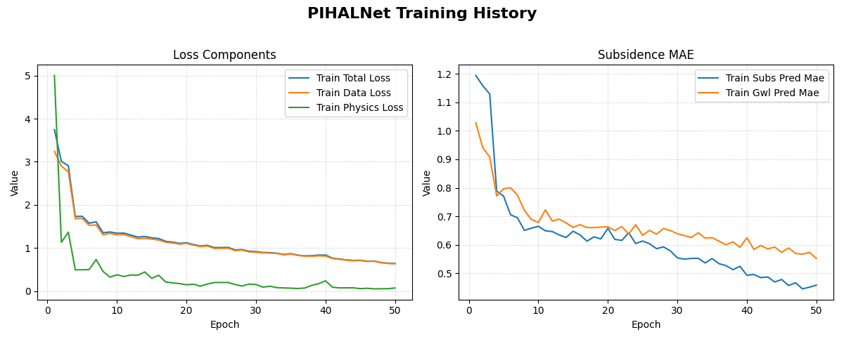
An example plot showing the training and validation loss and Mean Absolute Error (MAE) over epochs. This helps in diagnosing model fit and convergence.

In many cases you will want to monitor how well the network generalises while it trains. Below we create a second PIHALNet instance (model_val), split the synthetic dataset into an 80 / 20 train‑validation split, run model.fit with the validation_data argument, and finally plot both training and validation curves.

# 1. Prepare an explicit train / validation split
from tensorflow.data import AUTOTUNE

total_batches = int(
    tf.data.experimental.cardinality(dataset).numpy()
)
if total_batches < 2:
    # Not enough batches to split → fall back to 1 batch train + 1 batch val
    warnings.warn(
        "Dataset has a single batch; duplicating it for validation.",
        RuntimeWarning,
    )
    train_ds = dataset
    valid_ds = dataset.take(1).prefetch(AUTOTUNE)
else:
    val_batches = max(1, int(0.2 * total_batches))          # 20 % → validation
    train_ds = dataset.take(total_batches - val_batches)
    valid_ds = dataset.skip(total_batches - val_batches).prefetch(AUTOTUNE)

# 2. Instantiate a new PIHALNet model (identical hyper‑params)
model_val = PIHALNet(**fixed_model_params, **architectural_params)

model_val.compile(
    optimizer=Adam(learning_rate=1e-3, clipnorm=1.0),
    loss={
        "subs_pred": MeanSquaredError(name="subs_data_loss"),
        "gwl_pred":  MeanSquaredError(name="gwl_data_loss"),
    },
    metrics={
        "subs_pred": ["mae"],
        "gwl_pred":  ["mae"],
    },
    loss_weights={"subs_pred": 1.0, "gwl_pred": 0.8},
    lambda_pde=0.1,
)

# 3. Fit with validation_data; keep the History object
print("\nTraining model with validation monitoring...")
history_val = model_val.fit(
    train_ds,
    validation_data=valid_ds,
    epochs=50,
    verbose=1,
)
print("\nTraining finished.")

# 4. Plot both training and validation curves
from fusionlab.nn.models.utils import plot_history_in

print("\nPlotting training + validation history ...")

# Extend the metric groups to include their 'val_' counterparts
pihalnet_metrics_val = {
    "Loss Components": [
       "loss",  "total_loss", "data_loss", "physics_loss",
        "val_loss",'val_gwl_pred_loss', 'val_subs_pred_loss'
    ],
    "Subsidence MAE": [
        "subs_pred_mae", "gwl_pred_mae",
        "val_subs_pred_mae", "val_gwl_pred_mae",
        ]
}

plot_history_in(
    history_val,
    metrics=pihalnet_metrics_val,
    layout="subplots",
    title="PIHALNet Train & Valid History",
)

Example Output Plot:

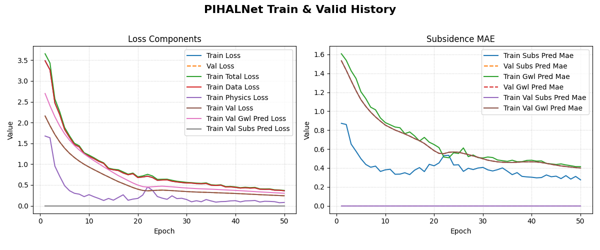
An example plot showing the training and validation loss and Mean Absolute Error (MAE) over epochs.

What you should see

• Left panel – total, data, and physics losses for both training (solid) and validation (dashed) sets.

• Right panel – MAE for subsidence and GWL; dashed curves represent validation MAE.

A widening gap between the solid and dashed curves would indicate over‑fitting; closely tracking curves suggest good generalisation.

Step 7: Make Predictions and Format for Visualization

After training, we use model.predict() and then structure the results into a long-format DataFrame suitable for forecast_view.

print("\nMaking predictions on the training data...")
predictions = model.predict(dataset)

# The output is a dictionary: {'subs_pred': ..., 'gwl_pred': ...}
# Let's format this into a pandas DataFrame.

# We will manually create the DataFrame for this exercise.
# In a real application, you might use a utility like
# `format_pihalnet_predictions`qqq.
# from fusionlab.nn.pinn.utils import format_pihalnet_predictions
# df_results = format_pihalnet_predictions (predictions)

all_rows = []
for i in range(BATCH_SIZE): # Iterate through each sample in the batch
    for j in range(FORECAST_HORIZON): # Iterate through each forecast step
        row = {
            'sample_idx': i,
            'forecast_step': j + 1,
            'coord_t': inputs['coords'][i, j, 0],
            'coord_x': inputs['coords'][i, j, 1],
            'coord_y': inputs['coords'][i, j, 2],
            'subsidence_pred': predictions['subs_pred'][i, j, 0],
            'subsidence_actual': targets['subs_pred'][i, j, 0],
            'GWL_pred': predictions['gwl_pred'][i, j, 0],
            'GWL_actual': targets['gwl_pred'][i, j, 0]
        }
        all_rows.append(row)

df_results = pd.DataFrame(all_rows)
print("\nFormatted prediction DataFrame (first 5 rows):")
print(df_results.head())

Expected Output:

Making predictions on the training data...
1/1 [==============================] - 0s 12ms/step

Formatted prediction DataFrame (first 5 rows):
   sample_idx  forecast_step  coord_t  ...  subsidence_actual  GWL_pred  GWL_actual
0           0              1      0.0  ...           0.144895  0.234190    0.341066
1           0              2      1.0  ...           0.489453 -0.349084    0.113474
2           0              3      2.0  ...           0.985650  0.326578    0.924694
3           0              4      3.0  ...           0.242055  0.388380    0.877339
4           0              5      4.0  ...           0.672136  0.464236    0.257942

[5 rows x 9 columns]

Step 7: Visualize the Forecast

Finally, we use forecast_view to visualize the spatial distribution of our predictions and compare them with the actuals.

print("\nVisualizing forecasts for 'subsidence'...")
plot_forecasts(
    forecast_df=df_results,
    target_name='subsidence', # We only plot subsidence
    kind='spatial',
    spatial_cols=('coord_x', 'coord_y'),
    dt_col='coord_t',
    horizon_steps = [1, 2, 3],
    max_cols=3, # Display 'Prediction' side-by-side
    cmap='viridis',
    axis_off=False,
    savefig=os.path.join(EXERCISE_OUTPUT_DIR, "pihalnet_exercise_forecast.png"),
    verbose=1
)

# we can use plot_forecast_by_step
from fusionlab.nn.pinn.utils import format_pihalnet_predictions
from fusionlab.plot.forecast import plot_forecast_by_step

# df_results = format_pihalnet_predictions (predictions)
# plot_forecast_by_step(df_results, steps = [1, 2, 3], value_prefixes =['subsidence'])

Expected Output:

Visualizing forecasts for 'subsidence'...
[INFO] Starting forecast visualization (kind='spatial')...
    [INFO]   Plotting for sample_idx: [0 1 2]
[INFO] Forecast visualization complete.

Expected Plot:

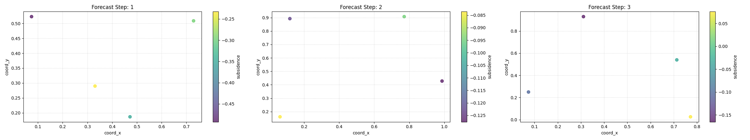
A grid of plots showing the spatial distribution of actual subsidence vs. predicted subsidence for each step in the forecast horizon.

Discussion of Exercise

In this exercise, you successfully:

• Configured and instantiated a complex PIHALNet model.

• Generated synthetic data that correctly separates past inputs (dynamic features) from the future prediction window (coords, future features, targets).

• Understood the importance of providing the model with coords that have a time dimension equal to the forecast_horizon.

• Trained the model and observed the data and physics loss components.

• Formatted predictions into a DataFrame and used forecast_view to visualize the results.

This workflow provides a solid foundation for applying PIHALNet and its associated tools to real-world spatio-temporal forecasting problems.