Basic Point Forecasting with Flexible TemporalFusionTransformer

This example demonstrates how to train the flexible TemporalFusionTransformer for a basic single-step, point forecasting task. We will use only dynamic (past observed) features for simplicity.

The workflow includes:

1. Generating simple synthetic time series data.

2. Preparing input sequences and targets using the create_sequences() utility.

3. Defining and compiling a TemporalFusionTransformer model configured for point forecasting.

4. Training the model for a few epochs.

5. Making a sample prediction and visualizing the results.

Prerequisites

Ensure you have fusionlab-learn and its dependencies installed:

pip install fusionlab-learn matplotlib

Step 1: Imports and Setup

We import standard libraries and the necessary components from fusionlab.

import numpy as np
import pandas as pd
import tensorflow as tf
import matplotlib.pyplot as plt
import warnings
import os

# FusionLab imports
from fusionlab.nn.transformers import TemporalFusionTransformer
from fusionlab.nn.utils import create_sequences
# Import loss for Keras to recognize if model was saved with it
from fusionlab.nn.losses import combined_quantile_loss

# Suppress warnings and TF logs for cleaner output
warnings.filterwarnings('ignore')
tf.get_logger().setLevel('ERROR')
if hasattr(tf, 'autograph'): # Check for autograph availability
    tf.autograph.set_verbosity(0)

print("Libraries imported and TensorFlow logs configured.")

Step 2: Generate Synthetic Data

A simple sine wave with added noise is created to serve as our univariate time series data.

time = np.arange(0, 100, 0.1)
amplitude = np.sin(time) + np.random.normal(
    0, 0.15, len(time)
    )
df = pd.DataFrame({'Value': amplitude})
print(f"Generated data shape: {df.shape}")
print("Sample of generated data:")
print(df.head())

Step 3: Prepare Sequences

The create_sequences() function transforms the flat time series into input-output pairs suitable for supervised learning. We’ll use the past 10 steps to predict the single next step.

sequence_length = 10    # Lookback window
forecast_horizon = 1    # Predict 1 step ahead (point forecast)
target_col_name = 'Value'

sequences, targets = create_sequences(
    df=df,
    sequence_length=sequence_length,
    target_col=target_col_name,
    forecast_horizon=forecast_horizon,
    verbose=0 # Suppress output from create_sequences
)

# Ensure data types are float32 for TensorFlow
sequences = sequences.astype(np.float32)
# Reshape targets for Keras: (Samples, Horizon, OutputDim=1)
# OutputDim is 1 because we predict one target variable ('Value')
targets = targets.reshape(
    -1, forecast_horizon, 1).astype(np.float32)

print(f"\nInput sequences shape (X): {sequences.shape}")
print(f"Target values shape (y): {targets.shape}")
# Example output:
# Input sequences shape (X): (990, 10, 1)
# Target values shape (y): (990, 1, 1)

Step 4: Define and Compile TFT Model

We instantiate the flexible TemporalFusionTransformer. Since we are only using dynamic features, static_input_dim and future_input_dim will be None (their default values). For point forecasting, quantiles is set to None.

# Get the number of features from the prepared sequences
num_dynamic_features = sequences.shape[-1]

model = TemporalFusionTransformer(
    dynamic_input_dim=num_dynamic_features,
    # static_input_dim defaults to None
    # future_input_dim defaults to None
    forecast_horizon=forecast_horizon,
    output_dim=1, # Predicting a single value per step
    hidden_units=16,        # Smaller for faster demo
    num_heads=2,            # Fewer heads for faster demo
    quantiles=None,         # Key for point forecasting
    num_lstm_layers=1,      # Example: 1 LSTM layer
    lstm_units=16           # Example: LSTM units
)
print("\nFlexible TemporalFusionTransformer instantiated for point forecast.")

# Compile the model with Mean Squared Error for point forecasting
model.compile(optimizer='adam', loss='mse')
print("Model compiled successfully with MSE loss.")

Step 5: Train the Model

The TemporalFusionTransformer expects inputs as a list of three elements: [static_inputs, dynamic_inputs, future_inputs]. Since we are only using dynamic inputs, the static and future inputs will be None.

# Prepare inputs for the model's fit method
# Order: [Static, Dynamic, Future] # since Static and Future are None
# we can pass only Dynamic, TFTFlex will handle it.
train_inputs = [sequences]

print("\nStarting model training (few epochs for demo)...")
history = model.fit(
    train_inputs, # Pass the 3-element list
    targets,      # Shape (Samples, Horizon, OutputDim)
    epochs=5,     # Increase for actual training
    batch_size=32,
    validation_split=0.2, # Keras uses last 20% for validation
    verbose=1             # Show training progress
)
print("Training finished.")
if history and history.history.get('val_loss'):
    print(f"Final validation loss: {history.history['val_loss'][-1]:.4f}")

Step 6: Make and Visualize Predictions

We’ll use a sample from the validation set to make a prediction and then plot the predictions against actual values.

# Prepare validation data for prediction
# Keras validation_split takes from the end of the data
num_samples = sequences.shape[0]
val_start_idx = int(num_samples * (1 - 0.2))

val_dynamic_inputs = sequences[val_start_idx:]
val_actuals_for_plot = targets[val_start_idx:]

# Package validation inputs in the [Dynamic] format since Static, and Future are None
val_inputs_list_for_plot = [val_dynamic_inputs]

print("\nMaking predictions on the validation set...")
val_predictions_scaled = model.predict(val_inputs_list_for_plot, verbose=0)
# val_predictions_scaled shape: (NumValSamples, Horizon, OutputDim)

print(f"Validation predictions shape: {val_predictions_scaled.shape}")
print("Sample prediction (first validation sample, first step):",
      val_predictions_scaled[0, 0, 0])

# --- Visualization ---
# Align time axis for plotting
# The target for sequence `i` corresponds to data point `time[i + sequence_length]`
# The validation data starts at `val_start_idx` in the `sequences` array.
plot_val_time_axis = time[
    val_start_idx + sequence_length : \
    val_start_idx + sequence_length + len(val_actuals_for_plot)
    ]

# Ensure plot_val_time_axis has the same length as predictions/actuals
# This can happen if len(val_actuals_for_plot) is small
num_plot_points = min(len(plot_val_time_axis), len(val_actuals_for_plot))

plt.figure(figsize=(14, 7))
# Plot a portion of original data for context
context_end_idx = val_start_idx + sequence_length + num_plot_points
plt.plot(time[:context_end_idx], amplitude[:context_end_idx],
         label='Original Data Context', alpha=0.6, color='lightblue')

# Plot actuals from validation set (first horizon step, first output dim)
plt.plot(plot_val_time_axis[:num_plot_points],
         val_actuals_for_plot[:num_plot_points, 0, 0],
         label=f'Actual Validation Data (H=1)',
         linestyle='--', marker='o', color='cyan')

# Plot predictions on validation set (first horizon step, first output dim)
plt.plot(plot_val_time_axis[:num_plot_points],
         val_predictions_scaled[:num_plot_points, 0, 0],
         label=f'Predicted Validation Data (H=1)',
         marker='D', color='orange', linestyle =':')

plt.title('Flexible TFT Point Forecast (Dynamic Input Only)')
plt.xlabel('Time')
plt.ylabel('Value')
plt.legend()
plt.grid(True)
plt.tight_layout()
# To save the figure:
# fig_path = os.path.join(output_dir_tft, "basic_tft_point_forecast.png")
# plt.savefig(fig_path)
# print(f"Plot saved to {fig_path}")
plt.show() # Display plot

print("\nBasic TFT point forecasting example complete.")

Example Output Plot:

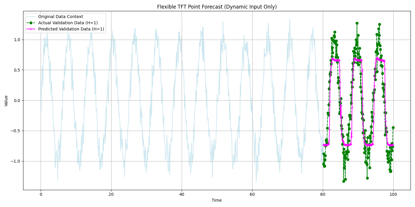
Visualization of the point forecast against actual validation data.

Explanations

1. Imports & Data: Standard setup using the flexible TemporalFusionTransformer.

2. Sequence Preparation: create_sequences() is used. Targets are reshaped to (NumSamples, Horizon, OutputDim).

3. Model Definition: The flexible TemporalFusionTransformer is instantiated. dynamic_input_dim is set. static_input_dim and future_input_dim default to None. quantiles=None ensures point forecasting. output_dim=1 is specified.

4. Model Compilation: Standard ‘mse’ loss.

5. Model Training:

   • Input Format: The input X is passed as a list [None, sequences, None]. This matches the expected [static_input, dynamic_input, future_input] order, with None for unused inputs.

6. Prediction: Input for prediction is also packaged as [None, sample_input_dynamic, None].

7. Visualization: The plot shows predictions against actuals on the validation set.