Exercise: Forecasting with a Pure Transformer

Welcome to this exercise on using the TimeSeriesTransformer. This guide will walk you through the complete process of building and training a pure transformer model for a multi-horizon, probabilistic time series forecasting task.

We will focus on demonstrating the model’s ability to handle multiple input types (static, dynamic, and future) and to generate quantile forecasts that capture prediction uncertainty.

Learning Objectives:

• Generate a synthetic time series dataset with static, dynamic past, and known future features.

• Prepare and shape the data into the list format required by the model: [static_data, dynamic_data, future_data].

• Instantiate the TimeSeriesTransformer and configure it for probabilistic (quantile) forecasting.

• Implement a custom quantile loss function and compile the model.

• Train the model and visualize the results, including the forecast distribution and uncertainty bounds.

Let’s get started!

Prerequisites

Ensure you have fusionlab-learn and its common dependencies installed.

pip install fusionlab-learn matplotlib scikit-learn

TimeSeriesTransformer

Step 1: Imports and Setup

First, we import all necessary libraries and set up our environment.

import os
import numpy as np
import tensorflow as tf
import matplotlib.pyplot as plt

# FusionLab imports
from fusionlab.nn.transformers import TimeSeriesTransformer

# Suppress warnings and TF logs for cleaner output
import warnings
warnings.filterwarnings('ignore')
tf.get_logger().setLevel('ERROR')

# Directory for saving any output images
EXERCISE_OUTPUT_DIR = "./pure_transformer_exercise_outputs"
os.makedirs(EXERCISE_OUTPUT_DIR, exist_ok=True)

print("Libraries imported and setup complete.")

Expected Output:

Libraries imported and setup complete.

Step 2: Generate and Prepare Synthetic Data

We’ll create a synthetic dataset and shape it into the three arrays required by the TimeSeriesTransformer: static, dynamic past, and known future features.

# Configuration
N_SAMPLES = 1000
PAST_STEPS = 30
HORIZON = 12
STATIC_DIM, DYNAMIC_DIM, FUTURE_DIM = 3, 4, 2
SEED = 42
np.random.seed(SEED)
tf.random.set_seed(SEED)

# --- Generate Dummy Data Arrays ---
static_features = np.random.randn(N_SAMPLES, STATIC_DIM)
dynamic_features = np.random.randn(N_SAMPLES, PAST_STEPS, DYNAMIC_DIM)
future_features = np.random.randn(N_SAMPLES, HORIZON, FUTURE_DIM)

# Create a simple target based on one of the dynamic features
targets = np.roll(dynamic_features[:, :, 0], -HORIZON, axis=1)[:, :HORIZON, np.newaxis] \
          + np.random.randn(N_SAMPLES, HORIZON, 1) * 0.5

# Split data into training and validation sets
val_split = -100
train_inputs = [arr[:val_split] for arr in [static_features, dynamic_features, future_features]]
val_inputs = [arr[val_split:] for arr in [static_features, dynamic_features, future_features]]
train_targets, val_targets = targets[:val_split], targets[val_split:]

print("Generated data shapes:")
print(f"  Training Inputs (static, dynamic, future): "
      f"{[x.shape for x in train_inputs]}")
print(f"  Training Targets: {train_targets.shape}")

Expected Output:

Generated data shapes:
  Training Inputs (static, dynamic, future): [(900, 3), (900, 30, 4), (900, 12, 2)]
  Training Targets: (900, 12, 1)

Step 3: Define, Compile, and Train the Model

Now, we instantiate the TimeSeriesTransformer. We will configure it for probabilistic forecasting by setting the quantiles parameter. This requires a corresponding quantile loss function for training.

# Define quantiles for probabilistic forecast
output_quantiles = [0.05, 0.5, 0.95] # p5, p50 (median), p95

# Instantiate the model
model = TimeSeriesTransformer(
    static_input_dim=STATIC_DIM,
    dynamic_input_dim=DYNAMIC_DIM,
    future_input_dim=FUTURE_DIM,
    output_dim=1,
    forecast_horizon=HORIZON,
    quantiles=output_quantiles,
    embed_dim=32,
    num_heads=4,
    ffn_dim=64,
    num_encoder_layers=2,
    num_decoder_layers=2
)

# Define a quantile loss function
def quantile_loss(y_true, y_pred):
    q = tf.constant(np.array(output_quantiles), dtype=tf.float32)
    e = y_true - y_pred
    # The tilted absolute loss function
    return tf.keras.backend.mean(
        tf.keras.backend.maximum(q * e, (q - 1) * e), axis=-1
    )

# Compile the model with the custom loss
model.compile(optimizer="adam", loss=quantile_loss)

# Train the model
print("\nStarting TimeSeriesTransformer training...")
history = model.fit(
    train_inputs,
    train_targets,
    validation_data=(val_inputs, val_targets),
    epochs=15,
    batch_size=128,
    verbose=0
)
print("Training complete.")
print(f"Final validation loss: {history.history['val_loss'][-1]:.4f}")

Expected Output:

Starting TimeSeriesTransformer training...
Training complete.
Final validation loss: 0.4041

Step 4: Visualize the Probabilistic Forecast

The key advantage of a quantile forecast is the ability to visualize uncertainty. We will plot the median prediction (p50) as our main forecast and shade the area between the lower (p5) and upper (p95) quantiles to represent the 90% prediction interval.

# Make predictions on the validation set
val_preds = model.predict(val_inputs)

# Select a single sequence from the validation set to plot
idx_to_plot = 25
median_pred = val_preds[idx_to_plot, :, 1] # 0.5 quantile is at index 1
lower_bound = val_preds[idx_to_plot, :, 0] # 0.05 quantile is at index 0
upper_bound = val_preds[idx_to_plot, :, 2] # 0.95 quantile is at index 2
actuals = val_targets[idx_to_plot, :, 0]

# --- Visualization ---
plt.figure(figsize=(12, 6))
time_axis = range(HORIZON)

# Plot uncertainty bounds
plt.fill_between(
    time_axis, lower_bound, upper_bound,
    color='orange', alpha=0.3, label='90% Prediction Interval'
)
# Plot actuals and median forecast
plt.plot(time_axis, actuals, 'o--', color='blue', label='Actual Values')
plt.plot(time_axis, median_pred, 'x-', color='red', label='Median Forecast (p50)')

plt.title('Probabilistic Forecast vs. Actuals (Validation Sample)')
plt.xlabel(f'Forecast Step (Horizon = {HORIZON} steps)')
plt.ylabel('Value')
plt.legend()
plt.grid(True, linestyle=':')
plt.tight_layout()
plt.show()

Expected Plot:

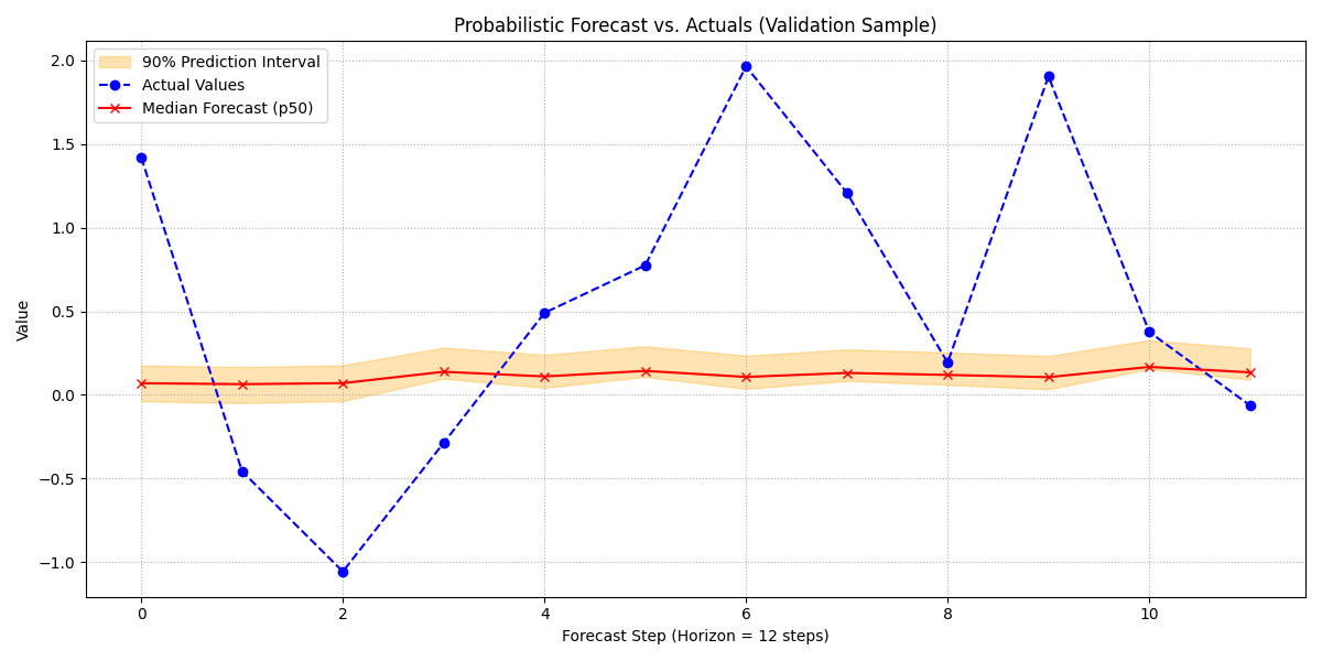
A plot showing the actual values, the median forecast, and the shaded 90% prediction interval. This visualizes not just what the model predicts, but also its confidence in that prediction.

Discussion of Exercise

Congratulations! You have successfully trained a pure transformer model for a complex, probabilistic forecasting task. In this exercise, you have learned to:

• Prepare data into the three-part list format (`[static, dynamic,

  future]`) required by the TimeSeriesTransformer.

• Configure the model to output quantile predictions for estimating

  uncertainty.

• Implement and use a custom quantile loss function for training.

• Visualize a probabilistic forecast, clearly showing the prediction

  interval around the median forecast.

This workflow demonstrates the power of pure attention-based models for capturing long-range dependencies and providing rich, uncertainty- aware forecasts.