Exercise: Physics-Informed Forecasting with PIHALNet & TransFlowSubsNet
Welcome to this comprehensive exercise on using the PIHALNet and
TransFlowSubsNet models. This guide will walk you through a
complete, real-world workflow for performing a multi-horizon,
probabilistic, physics-informed forecast for land subsidence and
groundwater level.
This is a deep-dive tutorial that covers every step from raw data ingestion to final visualization, demonstrating how to handle the complex data requirements of these advanced hybrid models.
Learning Objectives:
Load and preprocess a complex, real-world style dataset.
Perform feature engineering, including one-hot encoding and numerical scaling.
Use the
prepare_pinn_data_sequencesutility to transform a flat DataFrame into the specialized sequence format required by PINNs.Configure and train a hybrid model (
PIHALNetorTransFlowSubsNet) with both a data-driven loss and a physics-informed loss component.Set up callbacks for model checkpointing and early stopping.
Generate predictions on new data and format them into an interpretable DataFrame.
Visualize the multi-target, multi-horizon forecast results using the library’s specialized plotting functions.
Let’s get started!
Prerequisites
Ensure you have fusionlab-learn and its dependencies installed.
pip install fusionlab-learn "keras-tuner>=1.4.0" matplotlib scikit-learn
Step 0: Preamble & Configuration
First, we import all necessary libraries and define the main configuration parameters for our experiment. This central config block allows you to easily change the model, forecast period, or key hyperparameters for your own tests.
 1import os
 2import pandas as pd
 3import numpy as np
 4import tensorflow as tf
 5from sklearn.preprocessing import MinMaxScaler, OneHotEncoder
 6from tensorflow.keras.callbacks import EarlyStopping, ModelCheckpoint
 7
 8# --- FusionLab Imports ---
 9from fusionlab.datasets import fetch_zhongshan_data
10from fusionlab.nn.pinn.models import PIHALNet, TransFlowSubsNet
11from fusionlab.nn.pinn.utils import prepare_pinn_data_sequences
12from fusionlab.nn.losses import combined_quantile_loss
13from fusionlab.nn.models.utils import plot_history_in
14from fusionlab.nn.pinn.utils import format_pihalnet_predictions
15from fusionlab.plot.forecast import plot_forecasts
16
17# --- Main Configuration ---
18MODEL_NAME = 'TransFlowSubsNet'  # or 'PIHALNet'
19TRAIN_END_YEAR = 2022
20FORECAST_START_YEAR = 2023
21FORECAST_HORIZON_YEARS = 2
22TIME_STEPS = 4  # Lookback window
23QUANTILES = [0.1, 0.5, 0.9]
24EPOCHS = 20 # Use more epochs (e.g., 100+) for real results
25BATCH_SIZE = 256
26
27# --- PINN Configuration ---
28PDE_MODE_CONFIG = 'both' if MODEL_NAME == 'TransFlowSubsNet' else 'consolidation'
29LAMBDA_PDE_CONS = 1.0 # Weight for consolidation loss
30LAMBDA_PDE_GW = 1.0   # Weight for groundwater flow loss
31
32# --- Output Directory ---
33RUN_OUTPUT_PATH = f"./pihalnet_exercise_outputs/{MODEL_NAME}_run"
34os.makedirs(RUN_OUTPUT_PATH, exist_ok=True)
35print(f"Configuration set for model: {MODEL_NAME}")
36print(f"Output artifacts will be saved in: {RUN_OUTPUT_PATH}")
Expected Output 0:
Configuration set for model: TransFlowSubsNet
Output artifacts will be saved in: ./pihalnet_exercise_outputs/TransFlowSubsNet_run
Step 1: Load and Inspect the Dataset
We will load the Zhongshan dataset. The logic first tries to find a local, larger version of the file but will fall back to fetching the smaller, built-in version if it’s not found.
 1try:
 2    # For this exercise, we directly use the fetch utility
 3    print("Fetching Zhongshan dataset...")
 4    data_bunch = fetch_zhongshan_data()
 5    df_raw = data_bunch.frame
 6    print(f"Successfully loaded dataset. Shape: {df_raw.shape}")
 7except Exception as e:
 8    raise RuntimeError(f"Failed to fetch dataset: {e}")
 9
10print(df_raw.head())
Expected Output 1:
Fetching Zhongshan dataset...
Dataset 'zhongshan_2000.csv' found in package resource: fusionlab.datasets.data
Using cached version (also found in package): C:\Users\Daniel\fusionlab_data\zhongshan_2000.csv
Successfully loaded full data (1999 rows) from: C:\Users\Daniel\fusionlab_data\zhongshan_2000.csv
Loading full dataset (n_samples is None or '*').
Successfully loaded dataset. Shape: (1999, 14)
    longitude   latitude  ...  rainfall_category  subsidence
0  113.240334  22.476652  ...             Medium       15.51
1  113.215866  22.510025  ...             Medium       31.60
2  113.237984  22.494591  ...             Medium        8.09
3  113.219109  22.513433  ...             Medium       15.49
4  113.210678  22.536232  ...             Medium       14.02

[5 rows x 14 columns]
Step 2: Preprocessing - Feature Selection & Cleaning
We select the features relevant to our model and handle any missing values. For these models, we need coordinates (longitude, latitude), a time column (year), targets (subsidence, GWL), and other covariates.
 1from fusionlab.utils.data_utils import nan_ops
 2
 3TIME_COL, LON_COL, LAT_COL = 'year', 'longitude', 'latitude'
 4SUBSIDENCE_COL, GWL_COL = 'subsidence', 'GWL'
 5
 6# Select relevant features
 7features_to_use = [
 8    LON_COL, LAT_COL, TIME_COL, SUBSIDENCE_COL, GWL_COL,
 9    'rainfall_mm', 'geology', 'normalized_density'
10]
11df_selected = df_raw[features_to_use].copy()
12df_cleaned = nan_ops(df_selected, ops='sanitize', action='fill')
13print(f"NaNs after cleaning: {df_cleaned.isna().sum().sum()}")
Expected Output 2:
NaNs after cleaning: 0
Step 3: Preprocessing - Encoding & Scaling
Next, we convert categorical features like geology into a numerical format using one-hot encoding and scale all numerical features to a common range (0-1) using MinMaxScaler for stable training.
 1# --- Encoding Categorical Features ---
 2ohe = OneHotEncoder(sparse_output=False, handle_unknown='ignore')
 3encoded_data = ohe.fit_transform(df_cleaned[['geology']])
 4encoded_cols = ohe.get_feature_names_out(['geology'])
 5df_encoded = pd.DataFrame(encoded_data, columns=encoded_cols, index=df_cleaned.index)
 6df_processed = pd.concat([df_cleaned.drop('geology', axis=1), df_encoded], axis=1)
 7
 8# --- Create a numeric time coordinate for the PINN ---
 9TIME_COL_NUMERIC = "time_numeric"
10df_processed[TIME_COL_NUMERIC] = df_processed[TIME_COL] - df_processed[TIME_COL].min()
11
12# --- Scaling Numerical Features ---
13cols_to_scale = [c for c in df_processed.columns if c != TIME_COL]
14scaler = MinMaxScaler()
15df_scaled = df_processed.copy()
16df_scaled[cols_to_scale] = scaler.fit_transform(df_scaled[cols_to_scale])
17print("Categorical features encoded and numerical features scaled.")
18print(f"Final processed data shape: {df_scaled.shape}")
Expected Output 3:
Categorical features encoded and numerical features scaled.
Final processed data shape: (1999, 13)
Step 4: Define Feature Sets & Generate Sequences
This is a critical step where we tell our data preparation utility,
prepare_pinn_data_sequences, which columns to use for which input
stream (static, dynamic, etc.) and then generate the sequences.
 1# 1. Split data into training and testing periods
 2df_train_master = df_scaled[df_scaled[TIME_COL] <= TRAIN_END_YEAR]
 3df_test_master = df_scaled[df_scaled[TIME_COL] >= TRAIN_END_YEAR]
 4
 5# 2. Define feature lists
 6static_features_list = encoded_cols.tolist()
 7dynamic_features_list = [GWL_COL, 'rainfall_mm', 'normalized_density']
 8future_features_list = ['rainfall_mm'] # Assume rainfall forecast is known
 9
10# 3. Generate sequences
11inputs_train, targets_train = prepare_pinn_data_sequences(
12    df=df_train_master,
13    time_col=TIME_COL_NUMERIC,
14    lon_col=LON_COL, lat_col=LAT_COL,
15    subsidence_col=SUBSIDENCE_COL, gwl_col=GWL_COL,
16    dynamic_cols=dynamic_features_list,
17    static_cols=static_features_list,
18    future_cols=future_features_list,
19    group_id_cols=None, # [LON_COL, LAT_COL] Disable a group to treat as a big series
20    time_steps=TIME_STEPS,
21    forecast_horizon=FORECAST_HORIZON_YEARS,
22)
23print("\nTraining sequences generated.")
24for name, arr in inputs_train.items():
25    print(f"  Train Input '{name}' shape: {arr.shape if arr is not None else 'None'}")
Expected Output 4:
Training sequences generated.
  Train Input 'coords' shape: (1791, 2, 3)
  Train Input 'static_features' shape: (1791, 5)
  Train Input 'dynamic_features' shape: (1791, 4, 3)
  Train Input 'future_features' shape: (1791, 2, 1)
Step 5: Create tf.data.Dataset
We convert our NumPy sequence arrays into tf.data.Dataset objects
for efficient, high-performance training with TensorFlow.
 1# Standardize target keys to match model output names
 2targets_train_std = {
 3    'subs_pred': targets_train['subsidence'],
 4    'gwl_pred': targets_train['gwl']
 5}
 6
 7# Create the full dataset
 8full_dataset = tf.data.Dataset.from_tensor_slices((inputs_train, targets_train_std))
 9
10# Create train/validation split
11total_size = len(inputs_train['coords'])
12val_size = int(0.2 * total_size)
13train_size = total_size - val_size
14
15train_dataset = full_dataset.take(train_size).shuffle(train_size).batch(BATCH_SIZE).prefetch(tf.data.AUTOTUNE)
16val_dataset = full_dataset.skip(train_size).batch(BATCH_SIZE).prefetch(tf.data.AUTOTUNE)
17
18print(f"\nCreated training dataset ({train_size} samples) and validation dataset ({val_size} samples).")
Expected Output 5:
Created training dataset (1433 samples) and validation dataset (358 samples).
Step 6: Model Training
We now instantiate our chosen model, compile it with our composite loss function, and begin training.
 1# 1. Instantiate Model
 2ModelClass = TransFlowSubsNet if MODEL_NAME == 'TransFlowSubsNet' else PIHALNet
 3model = ModelClass(
 4    static_input_dim=inputs_train['static_features'].shape[-1],
 5    dynamic_input_dim=inputs_train['dynamic_features'].shape[-1],
 6    future_input_dim=inputs_train['future_features'].shape[-1],
 7    output_subsidence_dim=1, output_gwl_dim=1,
 8    forecast_horizon=FORECAST_HORIZON_YEARS,
 9    max_window_size=TIME_STEPS,
10    quantiles=QUANTILES,
11    pde_mode=PDE_MODE_CONFIG
12)
13
14# 2. Define Losses and Weights
15loss_dict = {'subs_pred': 'mse', 'gwl_pred': 'mse'}
16if QUANTILES:
17    loss_dict = {k: combined_quantile_loss(QUANTILES) for k in loss_dict}
18
19physics_loss_weights = {"lambda_cons": LAMBDA_PDE_CONS, "lambda_gw": LAMBDA_PDE_GW} \
20    if MODEL_NAME == 'TransFlowSubsNet' else {"lambda_physics": LAMBDA_PDE_CONFIG}
21
22# 3. Compile Model
23model.compile(
24    optimizer=tf.keras.optimizers.Adam(learning_rate=0.001),
25    loss=loss_dict,
26    loss_weights={'subs_pred': 1.0, 'gwl_pred': 0.5},
27    **physics_loss_weights
28)
29
30# 4. Train
31print(f"\nStarting {MODEL_NAME} training...")
32history = model.fit(
33    train_dataset,
34    validation_data=val_dataset,
35    epochs=EPOCHS,
36    callbacks=[EarlyStopping('val_loss', patience=10, restore_best_weights=True)]
37)
Expected Output 6:
Starting TransFlowSubsNet training...
Epoch 1/20
6/6 [==============================] - 30s 422ms/step - loss: 0.5286 - gwl_pred_loss: 0.4087 - subs_pred_loss: 0.3243 - total_loss: 0.5063 - data_loss: 0.5022 - physics_loss: 0.0041 - consolidation_loss: 0.0041 - gw_flow_loss: 2.9738e-07 - val_loss: 0.1235 - val_gwl_pred_loss: 0.2469 - val_subs_pred_loss: 0.0000e+00
Epoch 2/20
6/6 [==============================] - 0s 49ms/step - loss: 0.1974 - gwl_pred_loss: 0.1396 - subs_pred_loss: 0.1276 - total_loss: 0.1798 - data_loss: 0.1788 - physics_loss: 9.3386e-04 - consolidation_loss: 9.3376e-04 - gw_flow_loss: 1.0276e-07 - val_loss: 0.0356 - val_gwl_pred_loss: 0.0711 - val_subs_pred_loss: 0.0000e+00
...
Epoch 20/20
6/6 [==============================] - 0s 53ms/step - loss: 0.0295 - gwl_pred_loss: 0.0122 - subs_pred_loss: 0.0234 - total_loss: 0.0293 - data_loss: 0.0293 - physics_loss: 2.1400e-05 - consolidation_loss: 2.1400e-05 - gw_flow_loss: 2.2128e-11 - val_loss: 0.0043 - val_gwl_pred_loss: 0.0086 - val_subs_pred_loss: 0.0000e+00
Step 7: Visualize Results
Finally, we can use the plotting utilities to visualize the training history and the forecast results.
 1# Plot training history
 2plot_history_in(history, title=f'{MODEL_NAME} Training History')
 3
 4# Generate and plot forecasts on the validation set
 5val_inputs_batch, val_targets_batch = next(iter(val_dataset))
 6predictions = model.predict(val_inputs_batch)
 7
 8df_forecast = format_pihalnet_predictions(
 9    pihalnet_outputs=predictions,
10    y_true_dict=val_targets_batch,
11    target_mapping={'subs_pred': SUBSIDENCE_COL, 'gwl_pred': GWL_COL},
12    quantiles=QUANTILES,
13    forecast_horizon=FORECAST_HORIZON_YEARS,
14    model_inputs=val_inputs_batch,
15)
16
17if not df_forecast.empty:
18    plot_forecasts(
19        df_forecast,
20        target_name=SUBSIDENCE_COL,
21        quantiles=QUANTILES,
22        kind="temporal",
23        sample_ids="first_n",
24        num_samples=4
25    )
Expected Plot 7:
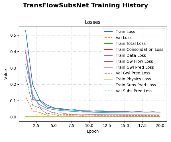
Visualization of TransFlowSubsNet traing loss history .
Discussion of Exercise
Congratulations! You have completed a full end-to-end workflow for a complex, hybrid physics-informed model. You have learned how to:
Take raw, tabular data and perform all necessary preprocessing steps.
Use the specialized
prepare_pinn_data_sequencesutility to create the multi-part input required by the models.Configure, compile, and train a
PIHALNetorTransFlowSubsNetmodel with a composite loss function.Evaluate the training process and visualize the final probabilistic forecasts.
This comprehensive process is a powerful template for applying these advanced models to your own scientific machine learning challenges.