Core Model Components

The advanced forecasting models in fusionlab-learn are not monolithic black boxes. They are sophisticated pipelines constructed from a rich ecosystem of specialized, reusable neural network layers, or components. Each component is designed to perform a specific, well-defined task, such as selecting important features, processing sequences, or fusing information with attention.

This section serves as a detailed guide to these fundamental building blocks, which are primarily located in the fusionlab.nn.components module.

Why Understanding Components Matters

A deep understanding of these components unlocks the full potential of the library and is crucial for several reasons:

• Deeper Insight: It allows you to move beyond simply using a model and start to understand how it works. You can reason about the flow of information and the mechanisms that give the architectures their predictive power.

• Enhanced Interpretability: Many components offer direct paths to interpretability. By inspecting the learned weights of a VariableSelectionNetwork, for instance, you can determine which input features the model found most predictive. Visualizing weights from an attention layer can reveal which past time steps were most influential for a given forecast.

• Advanced Customization & Research: The modular design is an open invitation for experimentation. Advanced users can easily “lego-brick” these components together to create novel architectures, test new hypotheses, or build a model tailored perfectly to the unique characteristics of a specific problem.

This guide provides an overview of the key components available, grouped thematically by their primary function.

Architectural Components

Activation

API Reference:

Activation

This is a simple utility layer that wraps standard Keras activation functions (e.g., ‘relu’, ‘elu’, ‘sigmoid’). Its primary purpose is to ensure consistent handling and serialization of activation functions within the fusionlab framework, particularly when models or custom layers using activations are saved and loaded. It internally uses tf.keras.activations.get() to resolve string names to callable functions.

While it can be used directly, users typically specify activations as strings (e.g., activation='relu') when initializing other layers (like GatedResidualNetwork), which then utilize this Activation layer or similar internal logic. Therefore, a direct code example is less illustrative here.

Positional Encoding

API Reference:

PositionalEncoding

Purpose: To inject information about the relative or absolute position of tokens (time steps) in a sequence. This is a critical component for any architecture that uses self-attention, such as the Transformer, TFT, and XTFT models. Standard self-attention mechanisms are permutation-invariant—they treat a sequence as an unordered “bag” of inputs. Positional encoding solves this by adding a unique, deterministic “signature” for each position, allowing the model to understand the order and distance between different points in time.

Functionality: This layer implements the classic sinusoidal positional encoding from the “Attention Is All You Need” paper [1]_. It creates a unique vector for each time step and adds it to the corresponding input feature embedding.

\[\text{Output}_t = \text{InputEmbedding}_t + PE_t\]

The positional encoding vector \(PE\) at each position pos is not a simple number but a vector whose elements are defined by sine and cosine functions of different frequencies:

\[PE_{(pos, 2i)} = \sin\left(\frac{pos}{10000^{2i/d_{\text{model}}}}\right)\]

\[PE_{(pos, 2i+1)} = \cos\left(\frac{pos}{10000^{2i/d_{\text{model}}}}\right)\]

where \(pos\) is the position in the sequence, \(i\) is the dimension index within the feature vector, and \(d_{\text{model}}\) is the total feature dimension (embed_dim). This formulation allows the model to easily learn to attend to relative positions, as the positional encoding of any time step can be represented as a linear function of any other.

For efficiency, the entire positional encoding matrix is pre-calculated up to a max_length and simply added to the input tensor during the forward pass.

Usage Context: This layer is typically applied to the sequence of temporal embeddings (derived from dynamic past and/or future inputs) after the initial feature projection but before the data enters the main temporal processing blocks, such as the encoder’s self-attention layers or a MultiScaleLSTM.

Code Example:

The following example demonstrates how to apply the layer and provides a visualization of the encoding matrix itself, which is a great way to build intuition.

import tensorflow as tf
import matplotlib.pyplot as plt
from fusionlab.nn.components import PositionalEncoding

# Dummy input tensor (Batch, TimeSteps, Features)
B, T, F = 4, 50, 128
input_sequence = tf.random.normal((B, T, F))

# Instantiate the layer
pos_encoding_layer = PositionalEncoding(max_length=200)

# Apply the layer to the input
output_sequence = pos_encoding_layer(input_sequence)

print(f"Input shape: {input_sequence.shape}")
print(f"Output shape after Positional Encoding: {output_sequence.shape}")
# The shape is unchanged.
assert input_sequence.shape == output_sequence.shape

# --- Visualize the Positional Encoding Matrix ---
# Extract the pre-calculated encoding matrix from the layer
pe_matrix = pos_encoding_layer.positional_encoding[0, :, :].numpy()

plt.figure(figsize=(10, 6))
cax = plt.pcolormesh(pe_matrix, cmap='viridis')
plt.gcf().colorbar(cax)
plt.title("Sinusoidal Positional Encoding Matrix")
plt.xlabel("Feature Dimension (i)")
plt.ylabel("Position in Sequence (pos)")
plt.show()

Expected Output:

Input shape: (4, 50, 128)
Output shape after Positional Encoding: (4, 50, 128)

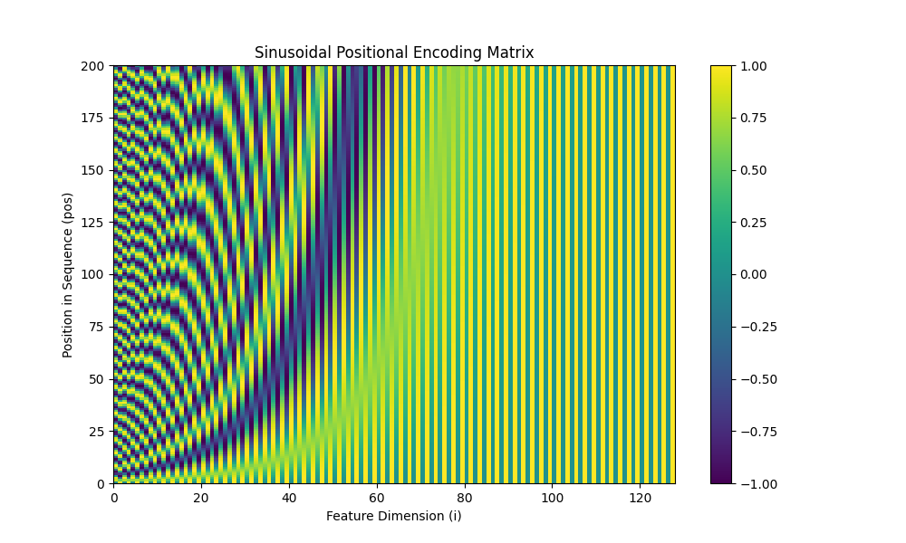
A visualization of the positional encoding matrix. Each row corresponds to a position in the sequence, and each column to a dimension in the feature vector. The plot clearly shows the unique sinusoidal patterns that give each time step its unique signature.

Gated Residual Network (GRN)

API Reference:

GatedResidualNetwork

Purpose: The Gated Residual Network (GRN) is arguably the most fundamental and versatile building block in the Temporal Fusion Transformer (TFT) family of models. It is a flexible and robust module for applying non-linear transformations to features, while ensuring the training process remains stable even in very deep networks.

It is designed to perform three key tasks simultaneously:

1. Non-linear Processing: To learn complex, non-linear relationships in the data.

2. Contextual Conditioning: To allow a transformation to be dynamically influenced by other information (e.g., static metadata).

3. Controlled Information Flow: To learn when to apply or skip the transformation entirely.

Architectural Deep Dive

The power of the GRN comes from the combination of several well-established deep learning concepts into a single, reusable component.

A diagram illustrating the flow of information through the Gated Residual Network, showing the main data path, the optional context addition, the gating mechanism, and the final residual connection. By Haizhou Du and Ziyi Duan, 2022, in Applied Intelligence (2022) 52:2496–2509) https://doi.org/10.1007/s10489-021-02532-x

Let’s break down the flow step-by-step:

1. (Optional) Context Addition: The GRN can be conditioned on an external context vector \(c\). If provided, this context is linearly projected to match the dimension of the primary input \(a\) and then added to it. This creates a contextualized input, \(a'\), allowing static information or other features to influence the transformation.

   \[a' = a + \text{Linear}_c(c)\]

   If no context is given, then \(a' = a\).

2. Main Transformation Path: The (contextualized) input \(a'\) is fed through a standard feed-forward path to learn a complex, non-linear representation. This typically involves a dense layer with a non-linear activation function like ELU or ReLU.

   \[\eta_1 = \text{ELU}(\text{Linear}_1(a'))\]

3. The Gating Mechanism: In parallel, the input \(a'\) is fed into a separate dense layer with a sigmoid activation function. The output of this layer, \(g\), is a vector of values between 0 and 1. This is the “gate.”

   \[g = \sigma(\text{Linear}_2(a'))\]

   This gate acts as an adaptive filter. It is element-wise multiplied with the output of the main transformation path. If an element in the gate is close to 0, it effectively “turns off” the corresponding part of the transformation. If it’s close to 1, it lets it pass through. This allows the GRN to learn to skip the non-linear transformation entirely in situations where a simple linear path is sufficient.

4. Residual (“Skip”) Connection & Normalization: Finally, the gated transformation is added back to the original input \(a\). This “skip connection,” popularized by ResNets, is critical for training deep networks as it prevents vanishing gradients and allows the model to easily learn identity mappings. If the input dimension of \(a\) differs from the GRN’s output dimension, a projection (Linear_p) is applied to \(a\) before the addition. The final result is passed through Layer Normalization.

   The complete formulation is:

   \[\text{GRN}(a, [c]) = \text{LayerNorm}\left(\text{proj}(a) + ( \eta_1 \odot g )\right)\]

Usage Context:

GRNs are the workhorse component used throughout the library’s advanced models for a variety of tasks:

• Processing static features to generate different context vectors.

• Acting as the core transformation block within the VariableSelectionNetwork.

• Serving as the position-wise feed-forward networks inside attention blocks.

• Enriching temporal features with static context.

Code Example:

import tensorflow as tf
from fusionlab.nn.components import GatedResidualNetwork

# --- Configuration ---
batch_size = 4
input_features = 32
hidden_units = 16 # The output dimension of the GRN

# --- Dummy input tensors ---
# Primary input
dummy_input = tf.random.normal((batch_size, input_features))
# Optional context vector (must match the GRN's output units)
dummy_context = tf.random.normal((batch_size, hidden_units))

# --- 1. Instantiate the GRN Layer ---
grn_layer = GatedResidualNetwork(
    units=hidden_units,
    dropout_rate=0.1,
    activation='elu'
)

# --- 2. Call without context ---
# The GRN applies its non-linear transformation to the input.
output_no_context = grn_layer(dummy_input, training=False)
print(f"GRN output shape (no context): {output_no_context.shape}")
assert output_no_context.shape == (batch_size, hidden_units)

# --- 3. Call with context ---
# The context vector influences the initial transformation.
output_with_context = grn_layer(
    dummy_input, context=dummy_context, training=False
)
print(f"GRN output shape (with context): {output_with_context.shape}")
assert output_with_context.shape == (batch_size, hidden_units)

# --- 4. Inspecting the layer ---
# The GRN is a standard Keras Layer with trainable weights.
print(f"\nNumber of trainable weights in the GRN: {len(grn_layer.trainable_weights)}")

Expected Output:

GRN output shape (no context): (4, 16)
GRN output shape (with context): (4, 16)

Number of trainable weights in the GRN: 11

VariableSelectionNetwork (VSN)

API Reference:

VariableSelectionNetwork

Purpose: To perform interpretable, instance-wise feature selection. In many complex forecasting problems, not all input variables are equally important, and their relevance can change depending on the context. For example, a rainfall feature might be highly relevant for predicting river levels during a storm but irrelevant during a drought.

The VSN is a powerful component designed to solve this problem. It allows the model to dynamically learn which features to pay attention to and which to ignore for each individual forecast, improving model performance by filtering out noise and providing valuable insights into which variables are driving the predictions.

Architectural Deep Dive

The VSN is much more sophisticated than a simple feature-dropping mechanism. It learns to create a weighted sum of rich, non-linear representations of each input variable. The architecture can be broken down into four key stages:

1. Feature-wise Non-linear Processing: First, instead of considering the raw input features directly, the VSN processes each input variable independently. Each variable \(\mathbf{x}_j\) from the input set is passed through its own dedicated GatedResidualNetwork (GRN).

   \[\tilde{\mathbf{x}}_j = \text{GRN}_j(\mathbf{x}_j, [c])\]

   This initial step is crucial. It allows the model to learn complex, non-linear patterns and transformations within each individual feature first, before deciding on its overall importance. This transformation can also be conditioned on an external context vector \(c\) (e.g., static features).

2. Learning Variable Importances: All the processed feature representations from the previous step, \(\{\tilde{\mathbf{x}}_1, \tilde{\mathbf{x}}_2, ..., \tilde{\mathbf{x}}_N\}\), are stacked together. This combined tensor is then fed into a separate, shared network (in this implementation, a single Dense layer followed by a GRN) to produce a single scalar logit, \(e_j\), for each variable. These logits represent the “un-normalized” importance of each feature.

3. Normalizing Weights with Softmax: To ensure the learned weights are interpretable and well-behaved, the logits \(\{e_j\}\) are passed through a Softmax function. This transforms them into the final importance weights, \(\alpha_j\), which are all positive and sum to 1.

   \[\alpha_j = \text{softmax}(e_j) = \frac{\exp(e_j)}{\sum_{k=1}^{N} \exp(e_k)}\]

   These weights, \(\alpha_j\), can be interpreted as the percentage of “attention” the model is paying to each input variable for a given prediction.

4. Weighted Summation: The final output of the VSN is a weighted sum of the rich, processed feature representations from Step 1, using the softmax weights from Step 3 as the coefficients.

   \[\text{VSN}(\mathbf{X}, [c]) = \sum_{j=1}^{N} \alpha_j \tilde{\mathbf{x}}_j\]

The output is a single, information-rich vector where the most relevant features (as determined by the network) have the greatest contribution.

Usage Context: VSNs are a hallmark of the TFT architecture. In fusionlab-learn, they are used in models like HALNet, XTFT, and PIHALNet as the first step in processing each of the three input types: static, dynamic past, and known future features. This allows the models to perform intelligent feature selection at every stage of the pipeline.

Code Example:

This example demonstrates how to use the VSN and, importantly, how to inspect the learned feature importances after a forward pass.

import tensorflow as tf
from fusionlab.nn.components import VariableSelectionNetwork

# --- Configuration ---
batch_size = 4
num_features = 8 # Number of input variables
units = 16       # Dimension of the GRN outputs

# --- 1. Create a dummy input tensor and a context vector ---
input_features = tf.random.normal((batch_size, num_features))
# Context vector can be used to influence the feature selection
context_vector = tf.random.normal((batch_size, units))

# --- 2. Instantiate and apply the VSN layer ---
vsn_layer = VariableSelectionNetwork(
    num_inputs=num_features,
    units=units,
    dropout_rate=0.1
)
# Pass both the inputs and the optional context
output_vector = vsn_layer(input_features, context=context_vector)

# --- 3. Inspect the results ---
print(f"Input shape: {input_features.shape}")
print(f"Output shape (weighted sum of features): {output_vector.shape}")

# The real value of VSN is its interpretability.
# We can access the learned weights for each feature.
feature_importances = vsn_layer.variable_importances_

# Shape is (Batch, NumFeatures, 1)
print(f"\nShape of learned feature importances: {feature_importances.shape}")

# Let's look at the importances for the first sample in the batch
sample_0_importances = tf.squeeze(feature_importances[0]).numpy()
print("\nLearned Feature Importances for Sample 0:")
for i, weight in enumerate(sample_0_importances):
    print(f"  Feature {i+1}: {weight:.3f}")

Expected Output:

Input shape: (4, 8)
Output shape (weighted sum of features): (4, 16)

Shape of learned feature importances: (4, 8, 1)

Learned Feature Importances for Sample 0:
  Feature 1: 0.008
  Feature 2: 0.091
  Feature 3: 0.347
  Feature 4: 0.004
  Feature 5: 0.029
  Feature 6: 0.019
  Feature 7: 0.497
  Feature 8: 0.005

Position-wise Feed-Forward Network (FFN)

API Reference:

PositionwiseFeedForward

The Position-wise Feed-Forward Network is a core component of the standard Transformer block, as introduced in the “Attention Is All You Need” paper. It is applied after the multi-head attention sub-layer and serves two primary purposes:

1. To introduce non-linearity, allowing the model to learn more complex functions.

2. To process and transform the context-rich representation of each position (or time step) independently.

How it Works

The “position-wise” nature is its defining characteristic. The exact same FFN, with the same learned weights, is applied to the feature vector at every single position in the input sequence. It does not mix information between positions; that task is handled by the preceding attention layer.

The network itself is a simple two-layer fully-connected network. The first layer expands the dimensionality of the input, and the second layer projects it back down.

\[\text{FFN}(x) = \text{Linear}_2(\text{activation}(\text{Linear}_1(x)))\]

Key Parameters

• `embed_dim`: The input and output dimensionality of the layer, which must match the model’s main embedding dimension (\(d_{model}\)).

• `ffn_dim`: The dimensionality of the inner, expanded hidden layer. A common practice is to set this to 4 * embed_dim.

• `activation`: The non-linear activation function (e.g., ‘relu’ or ‘gelu’) applied after the first linear transformation.

• `dropout_rate`: The dropout rate for regularization.

Usage Example

import tensorflow as tf
from fusionlab.nn.components import PositionwiseFeedForward

# 1. Create a dummy input tensor from a previous layer
# (batch_size, sequence_length, embed_dim)
input_tensor = tf.random.normal((32, 50, 128))

# 2. Instantiate the FFN layer
ffn_layer = PositionwiseFeedForward(
    embed_dim=128,  # Must match input's last dimension
    ffn_dim=512     # The expanded inner dimension
)

# 3. Pass the input through the layer
output_tensor = ffn_layer(input_tensor)

# The output shape is always the same as the input shape
print(f"Input Shape: {input_tensor.shape}")
print(f"Output Shape: {output_tensor.shape}")

Expected Output:

Input Shape: (32, 50, 128)
Output Shape: (32, 50, 128)

Gated Residual Network (GRN) vs. Position-wise FFN

In the XTFT architecture and the broader Temporal Fusion Transformer family, the standard Position-wise Feed-Forward Network(FFN) found in classic Transformers is deliberately replaced by a more sophisticated component: the Gated Residual Network (GRN). This choice is critical for handling the complexity and noise inherent in real-world time series data.

While an FFN provides essential non-linear transformation, a GRN enhances this process with two key mechanisms. First, it incorporates a gating mechanism, which acts like an intelligent information filter. This gate dynamically learns to control how much information flows through the layer, allowing the model to suppress noise or ignore irrelevant features at a specific time step. Second, the GRN has a built-in residual connection, which provides a direct path for information to bypass the transformation block. This stabilizes the training of deep networks by preventing the vanishing gradient problem and ensures the transformation is only applied if it is beneficial. By combining non-linear processing with learnable filtering and stable gradient flow, the GRN provides a much more robust and expressive building block than a standard FFN.

Comparison Table: FFN vs. GRN

Comparison Table: FFN vs. GRN

Feature	Position-wise Feed-Forward Network (FFN)	Gated Residual Network (GRN)	Significance & Benefit
Core Purpose	To apply a non-linear transformation to each position’s vector after attention.	To apply a controlled, non-linear transformation to each position’s vector.	GRN is more adaptive. Both add complexity, but the GRN’s transformation is conditional and can be skipped if not useful.
Basic Structure	Two linear (Dense) layers with a simple activation function (e.g., ReLU).	Two linear layers combined with a Gating Layer (GLU) and a residual (skip) connection.	GRN is more complex and powerful. The gating and skip connections are what give it superior performance.
Information Flow	Input data is always fully transformed by the network.	A gating mechanism learns to filter the input, deciding how much of the transformation to apply.	GRN can ignore noise. This is a major advantage in time series. The FFN lacks this dynamic filtering.
Residual Connections	Relies on an external residual connection applied after the layer in the main Transformer block.	The residual connection is an integral part of the GRN’s internal structure.	GRN has better gradient flow. Integrating the skip connection makes the component more robust and stable, especially in very deep networks.
Context Integration	Has no explicit mechanism to incorporate external context.	Explicitly designed to accept an optional context vector, which influences the gating behavior.	GRN is context-aware. This allows static features to directly influence the temporal processing at every time step, a key feature of the TFT architecture.
Origin	“Attention Is All You Need” (The original Transformer)	“Temporal Fusion Transformers for Interpretable Multi-horizon Time Series Forecasting”	The GRN is a specific innovation designed to overcome the limitations of a standard FFN for heterogeneous time series data.
When to Use	Excellent for general-purpose sequence processing where the main goal is transformation (e.g., NLP).	Superior for complex, noisy time series forecasting where filtering, context integration, and training stability are critical.	XTFT uses GRNs because they are better suited for the challenges of real-world forecasting data.

StaticEnrichmentLayer

API Reference:

StaticEnrichmentLayer

Purpose: To effectively infuse time-invariant static context into a sequence of time-varying temporal features. In many real-world problems, the nature of temporal patterns depends heavily on static attributes. For example, the sales seasonality for “Product A” might be completely different from “Product B”.

This layer is the mechanism that allows the model to learn these conditional relationships. It creates an “enriched” representation of the time series where the temporal dynamics are modulated by the static properties of the entity being forecast.

Architectural Deep Dive

The layer performs a three-step process to combine the two distinct types of information into a single, powerful representation.

1. Input Tensors: The layer takes two inputs:

   • Temporal Features (\(\mathbf{X}\)): A 3D tensor of shape (Batch, TimeSteps, Units), typically the output of a sequence encoder like an LSTM. It contains information about “what is happening over time.”

   • Static Context (\(\mathbf{c}\)): A 2D tensor of shape (Batch, Units), typicallythe output of processing static metadata. It contains information about “what entity we are looking at.”

2. Broadcasting the Static Context: The static context vector, which lacks a time dimension, must be made compatible with the temporal features. The layer achieves this by expanding its dimensions and tiling it across the time step axis, transforming \(\mathbf{c}\) into a new tensor \(\mathbf{C}\) of shape (Batch, TimeSteps, Units). Now, every time step in the sequence is associated with the same static context vector.

3. Concatenation and Gated Transformation: The broadcasted static context \(\mathbf{C}\) and the original temporal features \(\mathbf{X}\) are concatenated along the feature dimension. This creates a combined feature vector at each time step that contains both the original temporal information and the static context.

   This combined, richer tensor is then passed through a final GatedResidualNetwork (GRN). The GRN applies a powerful, learnable non-linear transformation to this concatenated input, allowing the model to discover the complex and subtle interactions between the static attributes and the temporal dynamics. The output is the final “enriched” sequence.

Usage Context:

This is a standard and critical component in Temporal Fusion Transformer (TFT) architectures. It is typically applied after the main sequence encoder (like an LSTM) and before the temporal self-attention layer. It serves as the primary mechanism for injecting static information deep into the temporal processing pipeline.

Code Example

import tensorflow as tf
from fusionlab.nn.components import StaticEnrichmentLayer

# --- Configuration ---
batch_size = 4
time_steps = 20
units = 64 # Dimension of features and context

# --- 1. Create Dummy Input Tensors ---
# Represents the output of a sequence encoder (e.g., LSTM)
temporal_features = tf.random.normal((batch_size, time_steps, units))
# Represents the processed static metadata
static_context_vector = tf.random.normal((batch_size, units))

# --- 2. Instantiate the Layer ---
enrichment_layer = StaticEnrichmentLayer(units=units, activation='relu')

# --- 3. Apply the layer ---
# The call signature is: call(temporal_features, static_context_vector)
enriched_features = enrichment_layer(temporal_features, static_context_vector)

# --- 4. Verify Shapes ---
print(f"Input temporal shape: {temporal_features.shape}")
print(f"Input static context shape: {static_context_vector.shape}")
print(f"Output enriched shape: {enriched_features.shape}")
# The output shape matches the temporal input shape, but its content
# is now enriched with static information.
assert enriched_features.shape == temporal_features.shape

Expected Output:

Input temporal shape: (4, 20, 64)
Input static context shape: (4, 64)
Output enriched shape: (4, 20, 64)

---

Input Processing & Embedding Layers

These layers are the first point of contact for the raw input data. They handle the initial transformation and embedding of various input types before they enter the main temporal processing stream of the models.

LearnedNormalization

API Reference:

LearnedNormalization

Purpose: To provide a dynamic, learnable alternative to traditional data preprocessing. In a typical workflow, you might scale your data using a tool like scikit-learn’s StandardScaler, which calculates a fixed mean and standard deviation from a training set. LearnedNormalization brings this process inside the model, allowing the network to learn the optimal normalization parameters as part of the end-to-end training process.

This approach gives the model the flexibility to adaptively determine the most suitable scale and shift for its input features based on what best minimizes the final loss function.

Benefits and Trade-offs

• Adaptability: If the data distribution is expected to shift between training and inference (a common issue known as data drift), a fixed scaler can become stale and suboptimal. By learning the normalization parameters, the model can be more robust to these variations.

• End-to-End Optimization: The normalization parameters (\(\mu\) and \(\sigma\)) are optimized with respect to the final model loss, just like any other weight. This means the model learns the exact scaling that helps it perform its task best, not just a generic standardization.

• Simpler Deployment: The normalization logic is part of the saved model itself. This eliminates the need to save, load, and manage separate scaler objects in a production pipeline.

• Trade-off: For simple, stationary datasets, a standard pre-calculated scaler is often sufficient and computationally lighter. LearnedNormalization is best suited for complex problems where you want to give the model maximum flexibility to control its internal representations.

How it Works

The layer is simple yet powerful. During its build phase, it creates two trainable weight vectors whose size matches the input feature dimension (\(D\)):

1. A mean vector (\(\mathbf{\mu}_{learned}\)), initialized to zeros.

2. A stddev vector (\(\mathbf{\sigma}_{learned}\)), initialized to ones.

During the forward pass, it applies standard normalization to the input tensor \(\mathbf{X}\) using these learned parameters:

\[\mathbf{X}_{norm} = \frac{\mathbf{X} - \mathbf{\mu}_{learned}}{\mathbf{\sigma}_{learned} + \epsilon}\]

Here, \(\epsilon\) is a small constant (e.g., 1e-6) added for numerical stability to prevent division by zero. These parameters are then updated via backpropagation during training.

Usage Context:

This layer is used in the XTFT model as an initial processing step for static input features, giving the model adaptive control over how it normalizes this crucial context.

Code Example:

import tensorflow as tf
from fusionlab.nn.components import LearnedNormalization

# --- Configuration ---
batch_size = 4
num_features = 5

# --- 1. Create a dummy input tensor ---
# Represents a batch of static features with non-zero mean and std
dummy_input = tf.random.normal(
    (batch_size, num_features), mean=10.0, stddev=2.0
)

# --- 2. Instantiate and apply the layer ---
learned_norm_layer = LearnedNormalization()
normalized_output = learned_norm_layer(dummy_input)

# --- 3. Inspect the layer's state and output ---
print("--- Layer State (Initial) ---")
print(f"Layer has {len(learned_norm_layer.trainable_weights)} trainable weight sets (mean and stddev)")
# The learned mean starts at 0
print(f"Initial Learned Mean (first 3 features): {learned_norm_layer.mean.numpy()[:3]}")
# The learned stddev starts at 1
print(f"Initial Learned Stddev (first 3 features): {learned_norm_layer.stddev.numpy()[:3]}")

print("\n--- Output Verification ---")
print(f"Input shape: {dummy_input.shape}")
print(f"Normalized output shape: {normalized_output.shape}")
# Initially, the output is just (input - 0) / 1, so stats are similar
print(f"Mean of normalized output (initial): {tf.reduce_mean(normalized_output):.2f}")
print(f"Stddev of normalized output (initial): {tf.math.reduce_std(normalized_output):.2f}")

Expected Output:

--- Layer State (Initial) ---
Layer has 2 trainable weight sets (mean and stddev)
Initial Learned Mean (first 3 features): [0. 0. 0.]
Initial Learned Stddev (first 3 features): [1. 1. 1.]

--- Output Verification ---
Input shape: (4, 5)
Normalized output shape: (4, 5)
Mean of normalized output (initial): 10.04
Stddev of normalized output (initial): 1.95

Note

The example shows that initially, the layer performs an identity-like transformation because its learned \(\mu\) and \(\sigma\) start at 0 and 1. Through backpropagation during model training, these weights would be updated to the optimal values for minimizing the overall model loss.

MultiModalEmbedding

API Reference:

MultiModalEmbedding

Purpose: To process multiple, distinct streams of time-varying data and fuse them into a single, unified representation. Advanced forecasting models often ingest different modalities of temporal data simultaneously, for example:

1. Dynamic Past Features: Historical data, like past sales or sensor readings.

2. Known Future Features: Data known in advance, like upcoming holidays, weather forecasts, or scheduled promotions.

These different input streams often have different numbers of features and represent different kinds of information. The MultiModalEmbedding layer is the component responsible for projecting each of these disparate modalities into a common, high-dimensional embedding space before they are fused together for downstream processing.

Architectural Deep Dive

The layer follows a simple yet powerful three-step process:

1. Multiple Input Streams: The layer is designed to accept a list of input tensors. Each tensor in the list represents a different modality, for example: [dynamic_input, future_input]. A key requirement is that while the number of features (the last dimension) can differ between modalities, their batch and time dimensions must be the same.

2. Independent Projection: The layer creates a separate, independent Dense layer for each input modality. When the model is called, each input tensor is passed through its own dedicated dense layer, which projects it from its original feature dimension to the common, unified embed_dim.

3. Concatenation: After each modality has been projected into the common embedding space, the resulting tensors are all concatenated along the last (feature) dimension. This creates a single, wide tensor that contains the learned representations of all input modalities, fused together and ready for the next stage of processing.

\[\begin{split}\mathbf{E}_{i} = \text{Dense}_i(\mathbf{M_i}) \quad \text{for each modality } i \\ \mathbf{H}_{out} = \text{Concat}\big( \mathbf{E}_1, \mathbf{E}_2, \dots, \mathbf{E}_n \big)\end{split}\]

Usage Context: This layer is used at the beginning of the temporal processing pipeline in models like XTFT. It is one of the first steps in creating a unified representation from the various time-varying inputs before they are passed to components like PositionalEncoding or the main model encoder.

Code Example:

This example demonstrates how to embed two different input modalities (e.g., dynamic past features and known future features) into a single, concatenated tensor.

import tensorflow as tf
from fusionlab.nn.components import MultiModalEmbedding

# --- Configuration ---
batch_size = 32
time_steps = 10
embed_dim_per_modality = 64

# --- 1. Create Dummy Input Tensors for Two Modalities ---
# Represents historical data with 16 features
dynamic_input = tf.random.normal((batch_size, time_steps, 16))
# Represents future data with 8 features
future_input = tf.random.normal((batch_size, time_steps, 8))

# --- 2. Instantiate and Apply the Layer ---
mm_embedding_layer = MultiModalEmbedding(embed_dim=embed_dim_per_modality)

# The layer accepts a list of the input tensors
fused_embeddings = mm_embedding_layer([dynamic_input, future_input])

# --- 3. Verify Shapes ---
print(f"Shape of dynamic input: {dynamic_input.shape}")
print(f"Shape of future input:  {future_input.shape}")
print(f"Shape of fused output:  {fused_embeddings.shape}")

# The final feature dimension is the sum of the embed_dim for each modality
expected_output_dim = embed_dim_per_modality * 2
print(f"\nExpected output feature dimension: {expected_output_dim}")
assert fused_embeddings.shape[-1] == expected_output_dim

Expected Output:

Shape of dynamic input: (32, 10, 16)
Shape of future input:  (32, 10, 8)
Shape of fused output:  (32, 10, 128)

Expected output feature dimension: 128

---

Sequence Processing Layers

These layers are designed to process temporal sequences to capture dependencies, patterns, and contextual information over time.

MultiScaleLSTM

API Reference:

MultiScaleLSTM

Purpose: To analyze temporal patterns in a sequence at multiple time resolutions simultaneously. Real-world time series often contain a mixture of patterns that occur over different time horizons—for example, intraday fluctuations, daily seasonality, and weekly or monthly trends. A single LSTM processing data step-by-step can struggle to effectively capture all these different frequencies at once.

The MultiScaleLSTM layer solves this by acting like a set of parallel “lenses,” each viewing the same input time series at a different resolution or “zoom level.” By applying multiple LSTMs to sub-sampled versions of the input, it allows the model to concurrently learn short-term, medium-term, and long-term dynamics, creating a rich, multi-resolution summary of the temporal features.

Architectural Deep Dive

The layer internally manages a collection of standard Keras LSTM layers and processes the input sequence through them in parallel.

1. Input: The layer receives a single input time series tensor, \(\mathbf{X}\), of shape (Batch, TimeSteps, Features).

2. Parallel Sub-sampling: For each integer scale \(s\) provided in the scales list (e.g., [1, 3, 7]), the layer creates a new, shorter sequence by taking every \(s\)-th time step from the original input.

   \[\mathbf{X}_s = \mathbf{X}[:, ::s, :]\]

   For example, a scale of 1 uses the original sequence, while a scale of 7 would effectively create a sequence of weekly data points from a daily input.

3. Independent LSTM Processing: Each of these new, sub-sampled sequences (\(\mathbf{X}_1, \mathbf{X}_3, \mathbf{X}_7\), etc.) is fed into its own independent LSTM layer. While all LSTMs in the set share the same number of lstm_units, they each have their own separate, trainable weights, allowing them to specialize in finding patterns at their assigned scale.

4. Output Aggregation: The final output format is controlled by the return_sequences parameter, catering to two primary use cases:

   • Feature Extraction (`return_sequences=False`): In this mode, each LSTM processes its sub-sampled sequence and returns only its final hidden state, a single vector of shape \((B, \text{lstm_{units}})\) that summarizes the patterns found at that scale. All of these summary vectors are then concatenated along the feature dimension. This creates a single, rich feature vector that represents the temporal dynamics across all scales.

     \[\text{Output} \in \mathbb{R}^{B, \text{lstm}_{units} \times |\text{scales}|}\]

   • Encoder Mode (return_sequences=True): In this mode, each LSTM returns the full sequence of hidden states for its sub-sampled input. Because each sequence has a different length (\(\approx T/s\)), the layer returns a list of output tensors. This mode is used when the layer is part of an encoder, and a downstream attention mechanism needs to attend to the full contextualized output of each scale.

Usage Context: This layer is a key component of the ‘hybrid’ encoder architecture within BaseAttentive and its children, like HALNet and XTFT. The utility function aggregate_multiscale() is often used subsequently to combine the list of tensors produced when return_sequences=True.

Code Example:

import tensorflow as tf
from fusionlab.nn.components import MultiScaleLSTM

# --- Configuration ---
batch_size = 4
time_steps = 30
features = 8
lstm_units = 16
# Analyze patterns at original, 5-step, and 10-step resolutions
scales = [1, 5, 10]

# --- Create a dummy input tensor ---
dummy_input = tf.random.normal((batch_size, time_steps, features))
print(f"Input shape: {dummy_input.shape}")

# --- Example 1: Return only final hidden states ---
# This mode is for creating a single feature vector summary.
ms_lstm_final_state = MultiScaleLSTM(
    lstm_units=lstm_units,
    scales=scales,
    return_sequences=False # Default behavior
)
final_states_concat = ms_lstm_final_state(dummy_input)
print("\n--- Return Final States ---")
print(f"Output shape: {final_states_concat.shape}")
print(f"(Expected: B, units * num_scales -> {batch_size}, {lstm_units * len(scales)})")

# --- Example 2: Return full sequences ---
# This mode is for encoder backbones.
ms_lstm_sequences = MultiScaleLSTM(
    lstm_units=lstm_units,
    scales=scales,
    return_sequences=True
)
output_sequences_list = ms_lstm_sequences(dummy_input)
print(f"\n--- Return Full Sequences ---")
print(f"Output type: {type(output_sequences_list)}")
print(f"Number of output sequences in list: {len(output_sequences_list)}")
for i, seq in enumerate(output_sequences_list):
    print(f"  Shape of sequence for scale={scales[i]}: {seq.shape}")

Expected Output:

Input shape: (4, 30, 8)

--- Return Final States ---
Output shape: (4, 48)
(Expected: B, units * num_scales -> 4, 48)

--- Return Full Sequences ---
Output type: <class 'list'>
Number of output sequences in list: 3
  Shape of sequence for scale=1: (4, 30, 16)
  Shape of sequence for scale=5: (4, 6, 16)
  Shape of sequence for scale=10: (4, 3, 16)

DynamicTimeWindow

API Reference:

DynamicTimeWindow

Purpose: To apply a “recency filter” to a sequence, selecting a fixed-size window containing only the most recent time steps. In deep, multi-stage forecasting models like XTFT, information from the distant past is often already processed and summarized by earlier layers (e.g., MultiScaleLSTM or MemoryAugmentedAttention ).

The DynamicTimeWindow layer allows the final prediction stages of the model to focus on the most immediate and often most relevant temporal context, ensuring that the final output is not overwhelmed by older, already-processed information.

How It Works

Architecturally, this is one of the simplest layers, but it serves an important strategic role. It performs a single, highly-optimized slicing operation on the input tensor.

Given an input tensor representing a time series with \(T\) steps (shape \((B, T, D)\)), it returns only the last \(W\) steps, where \(W\) is the max_window_size.

\[\text{Output} = \text{Input}[:, -W:, :]\]

A key behavior is its robustness to variable sequence lengths. If the input sequence length \(T\) is less than or equal to the specified max_window_size, the layer simply returns the entire, unmodified input sequence.

Usage Context: This layer is used within the XTFT model as one of the final steps in the temporal processing pipeline. It is typically applied after the main attention fusion stages but before the final temporal aggregation (controlled by final_agg) and the MultiDecoder.

This placement allows the model to first build a rich, long-range context using attention, and then use this layer to zoom in on the most recent, highly-contextualized features just before generating the final forecast. It provides a mechanism to balance long-term context with short-term recency.

Code Example:

import tensorflow as tf
from fusionlab.nn.components import DynamicTimeWindow

# --- Configuration ---
batch_size = 4
time_steps = 30    # The full length of the input sequence
features = 8
window_size = 10   # We want to select only the last 10 steps

# --- 1. Create a dummy input tensor ---
# This could be the output of a complex attention fusion layer
dummy_input = tf.random.normal((batch_size, time_steps, features))

# --- 2. Instantiate and apply the layer ---
time_window_layer = DynamicTimeWindow(max_window_size=window_size)
windowed_output = time_window_layer(dummy_input)

# --- 3. Verify Shapes ---
print(f"Input shape: {dummy_input.shape}")
print(f"Output windowed shape: {windowed_output.shape}")

# The time dimension is now sliced to the window_size
assert windowed_output.shape[1] == window_size
# The batch and feature dimensions remain unchanged
assert windowed_output.shape[0] == batch_size
assert windowed_output.shape[2] == features

Expected Output:

Input shape: (4, 30, 8)
Output windowed shape: (4, 10, 8)

---

Attention Mechanisms

Attention layers are a powerful tool in modern deep learning, allowing models to dynamically weigh the importance of different parts of the input when producing an output or representation. Instead of treating all inputs equally, attention mechanisms learn to focus on the most relevant information for the task at hand. fusionlab-learn utilizes several specialized attention components, often based on the core concepts described below.

Core Concept: Scaled Dot-Product Attention

The fundamental building block for many attention mechanisms is the scaled dot-product attention [1]_. It operates on three sets of vectors: Queries (\(\mathbf{Q}\)), Keys (\(\mathbf{K}\)), and Values (\(\mathbf{V}\)).

1. Similarity Scoring: The relevance or similarity between each Query vector and all Key vectors is computed using the dot product.

2. Scaling: The scores are scaled down by dividing by the square root of the key dimension (\(d_k\)) to stabilize gradients during training.

3. Weighting (Softmax): A softmax function is applied to the scaled scores to obtain attention weights, which sum to 1. These weights indicate how much focus should be placed on each Value vector.

4. Weighted Sum: The final output is the weighted sum of the Value vectors, using the computed attention weights.

The formula is:

\[\text{Attention}(\mathbf{Q}, \mathbf{K}, \mathbf{V}) = \text{softmax}\left(\frac{\mathbf{Q}\mathbf{K}^T}{\sqrt{d_k}}\right)\mathbf{V}\]

Here, \(\mathbf{Q} \in \mathbb{R}^{T_q \times d_q}\), \(\mathbf{K} \in \mathbb{R}^{T_k \times d_k}\), and \(\mathbf{V} \in \mathbb{R}^{T_v \times d_v}\) (where \(T_k = T_v\) usually holds, and often \(d_q = d_k\)). The output has dimensions \(\mathbb{R}^{T_q \times d_v}\).

Multi-Head Attention

Instead of performing a single attention calculation, Multi-Head Attention [1]_ allows the model to jointly attend to information from different representational subspaces at different positions.

1. Projection: The original Queries, Keys, and Values are linearly projected \(h\) times (where \(h\) is the number of heads) using different, learned linear projections (\(\mathbf{W}^Q_i, \mathbf{W}^K_i, \mathbf{W}^V_i\) for head \(i=1...h\)).

2. Parallel Attention: Scaled dot-product attention is applied in parallel to each of these projected versions, yielding \(h\) different output vectors (\(head_i\)).

   \[head_i = \text{Attention}(\mathbf{Q}\mathbf{W}^Q_i, \mathbf{K}\mathbf{W}^K_i, \mathbf{V}\mathbf{W}^V_i)\]

3. Concatenation: The outputs from all heads are concatenated together.

4. Final Projection: The concatenated output is passed through a final linear projection (\(\mathbf{W}^O\)) to produce the final Multi-Head Attention output.

\[\text{MultiHead}(\mathbf{Q}, \mathbf{K}, \mathbf{V}) = \text{Concat}(head_1, ..., head_h)\mathbf{W}^O\]

This allows each head to potentially focus on different aspects or relationships within the data.

Self-Attention vs. Cross-Attention

• Self-Attention: When \(\mathbf{Q}, \mathbf{K}, \mathbf{V}\) are all derived from the same input sequence (e.g., finding relationships within a single time series).

• Cross-Attention: When the Query comes from one sequence and the Keys/Values come from a different sequence (e.g., finding relationships between past inputs and future inputs, or between dynamic and static features).

The specific attention components provided by fusionlab-learn build upon or adapt these fundamental concepts for various purposes within time series modeling.

ExplainableAttention

API Reference:

ExplainableAttention

Purpose: To serve as a diagnostic and interpretability tool for understanding a model’s inner workings. While standard attention layers process an input sequence and return a transformed sequence, this layer “opens up the black box” by exposing the raw attention weights.

Its goal is to directly answer the question: “For a given time step, which other time steps did the model focus on?” This provides a direct path to understanding the model’s reasoning and debugging its behavior.

Architectural Deep Dive

This layer is a very thin wrapper around the standard Keras MultiHeadAttention layer, with a crucial change in its call method.

1. Input: It receives a single input tensor \(\mathbf{X}\) of shape (Batch, TimeSteps, Features).

2. Self-Attention: It calls the internal MultiHeadAttention layer by passing the same input \(\mathbf{X}\) as the query, key, and value. This signifies a self-attention operation, where the sequence attends to itself.

3. Return Scores: Crucially, it sets the return_attention_scores argument to True. When called this way, the underlying Keras layer returns a tuple (weighted_output, attention_scores). The ExplainableAttention layer discards the first element and returns only the attention_scores.

The output is a 4D tensor of shape \((B, H, T_q, T_k)\), where:

• \(B\): Batch size

• \(H\): Number of attention heads

• \(T_q\): Query sequence length (the “target” time steps)

• \(T_k\): Key sequence length (the “source” time steps)

For self-attention, \(T_q\) and \(T_k\) are the same.

Usage Context & Interpretation This layer is primarily intended for offline analysis, debugging, and visualization, not as a component in a model’s main predictive path. With the output attention scores, you can:

• Visualize Attention Heatmaps: For a single head in a single sample, you get a \((T, T)\) matrix that can be plotted as a heatmap to see which time steps attended to which others.

• Identify Important Timesteps: For a given prediction, you can find which past time steps received the highest attention weights, revealing if the model is focusing on recency, seasonality, or specific past events.

• Debug Model Behavior: If a model produces an unexpected forecast, visualizing the attention scores can reveal if it was “looking” at irrelevant or noisy parts of the input history.

Code Example:

This example demonstrates how to get the attention scores for a sequence attending to itself.

import tensorflow as tf
import numpy as np
from fusionlab.nn.components import ExplainableAttention

# --- Configuration ---
batch_size = 4
time_steps = 20
key_dim = 64
num_heads = 2

# 1. Create a dummy input sequence
input_sequence = tf.random.normal((batch_size, time_steps, key_dim))

# 2. Instantiate and apply the layer for self-attention
explainable_attn_layer = ExplainableAttention(
    num_heads=num_heads,
    key_dim=key_dim
)
attention_scores = explainable_attn_layer(input_sequence)

# 3. Verify and interpret the output shape
print(f"Input sequence shape: {input_sequence.shape}")
print(f"Output attention scores shape: {attention_scores.shape}")
print("(Batch, Heads, Query_Steps, Key_Steps)")

# 4. Example of inspecting the scores for one head
# Get the scores for the first sample in the batch and the first head
single_head_scores = attention_scores[0, 0, :, :].numpy()
print(f"\nShape of scores for a single head: {single_head_scores.shape}")
# This (20, 20) matrix shows how each of the 20 time steps
# attended to every other time step.

Expected Output:

Input sequence shape: (4, 20, 64)
Output attention scores shape: (4, 2, 20, 20)
(Batch, Heads, Query_Steps, Key_Steps)

Shape of scores for a single head: (20, 20)

CrossAttention

API Reference:

CrossAttention

Purpose: To enable a model to fuse information and model the interaction between two distinct input sequences. If self-attention is about a sequence “understanding itself” by finding internal relationships, cross-attention is about one sequence “asking questions” and finding the most relevant answers within a second, different sequence.

Its primary role is to allow a query sequence to selectively extract and integrate the most relevant information from a key/value context sequence. This is the fundamental mechanism that allows an encoder-decoder model to work, enabling the decoder to focus on the most important parts of the encoded input when generating an output.

Architectural Deep Dive

The layer takes two sequences, source1 and source2, and performs the following steps:

1. Input Projections:

   Since the two input sequences, \(\mathbf{S}_1\) (from source1) and \(\mathbf{S}_2\) (from source2), may have different feature dimensions, they are first passed through independent Dense layers to project them into a common, shared dimensionality, \(d_{model}\). This process creates the three essential inputs for the attention mechanism: the Query, Key, and Value matrices.

   • Query: \(\mathbf{Q} = \mathbf{S}_1 \mathbf{W}_q\) (derived from source1)

   • Key: \(\mathbf{K} = \mathbf{S}_2 \mathbf{W}_k\) (derived from source2)

   • Value: \(\mathbf{V} = \mathbf{S}_2 \mathbf{W}_v\) (derived from source2)

   Note: In this implementation, the projection weights for the Key and Value are shared, meaning \(\mathbf{W}_k = \mathbf{W}_v\).

2. Scaled Dot-Product Attention:

   The core attention mechanism is now applied. For each element (e.g., time step) in the query sequence \(\mathbf{Q}\), a similarity score is computed against every element in the key sequence \(\mathbf{K}\). These scores are then normalized into attention weights, which are used to create a weighted average of the elements in the value sequence \(\mathbf{V}\).

   \[\text{Attention}(\mathbf{Q}, \mathbf{K}, \mathbf{V}) = \text{softmax}\left(\frac{\mathbf{Q}\mathbf{K}^T}{\sqrt{d_k}}\right)\mathbf{V}\]

   The result is a new sequence where each element is a summary of the most relevant parts of \(\mathbf{S}_2\) from the perspective of the corresponding element in \(\mathbf{S}_1\).

3. Multi-Head Execution: This entire process is performed in parallel across multiple “heads,” each with its own set of learned projection matrices (\(\mathbf{W}_q^i, \mathbf{W}_k^i, \mathbf{W}_v^i\)). This allows different heads to focus on different types of relationships between the two sequences simultaneously. The final outputs from all heads are then concatenated and linearly projected to produce the final result.

Self-Attention vs. Cross-Attention

The following table clarifies the key differences between these two fundamental attention types.

Self-Attention vs. Cross-Attention

Aspect	Self-Attention	Cross-Attention
Core Purpose	To find relationships within a single sequence. Answers: “Which other parts of this sequence are relevant to the current position?”	To fuse information between two different sequences. Answers: “Which parts of the second sequence are relevant to the first?”
Inputs (Q, K, V)	Query, Key, and Value are all derived from the same input sequence. \(\mathbf{Q, K, V} = f(\mathbf{S}_1)\)	Query is from one sequence, Key and Value are from a second sequence. \(\mathbf{Q}=f(\mathbf{S}_1)\), \(\mathbf{K, V}=g(\mathbf{S}_2)\)
Typical Use Case	Encoder layers in a Transformer; refining representations by capturing internal context.	The bridge between the encoder and decoder in a Transformer; fusing multi-modal data.
Information Flow	Internal. Enriches each element with context from its own sequence.	Directional. Transfers relevant information from the Key/Value sequence to the Query sequence.
Example Application	In a sentence, determining that the word “it” refers to “the animal” from earlier in the same sentence.	In translation, a decoder generating a French word (query) attends to the entire English source sentence (key/value).

Usage Context: Cross-attention is the cornerstone of encoder-decoder architectures. In models like XTFT and HALNet, it is used in the decoder to allow the future forecast context (the query) to attend to the rich summary of all historical information produced by the encoder (the key and value).

Code Example:

import tensorflow as tf
from fusionlab.nn.components import CrossAttention

# --- Configuration ---
batch_size = 4
query_seq_len = 10   # Length of the "asking" sequence
key_val_seq_len = 15 # Length of the "answering" sequence
query_features = 8
key_val_features = 12
units = 16           # Target dimension for attention
num_heads = 2

# --- 1. Create Dummy Input Tensors ---
# This sequence asks the questions (e.g., decoder context)
query_sequence = tf.random.normal((batch_size, query_seq_len, query_features))
# This sequence provides the context to be searched (e.g., encoder output)
context_sequence = tf.random.normal((batch_size, key_val_seq_len, key_val_features))

# --- 2. Instantiate and Apply the Layer ---
cross_attn_layer = CrossAttention(units=units, num_heads=num_heads)

# The layer expects a list: [query, context]
output = cross_attn_layer([query_sequence, context_sequence])

# --- 3. Verify Shapes ---
print(f"Query (source 1) shape: {query_sequence.shape}")
print(f"Context (source 2) shape: {context_sequence.shape}")
print(f"Output context vector shape: {output.shape}")

# The output shape aligns with the query sequence length and the layer's units.
# It has shape (B, T_query, units)
assert output.shape == (batch_size, query_seq_len, units)

Expected Output:

Query (source 1) shape: (4, 10, 8)
Context (source 2) shape: (4, 15, 12)
Output context vector shape: (4, 10, 16)

TemporalAttentionLayer

API Reference:

TemporalAttentionLayer

Purpose: To serve as the primary temporal processing block within the Temporal Fusion Transformer architecture. Its core purpose is to perform contextualized self-attention. This powerful mechanism allows each time step in a sequence to look at all other past time steps to find relevant information, but the “way” it looks (i.e., the query it forms) is dynamically influenced by static, time-invariant context.

This allows the model to answer questions like: “Given that I am forecasting for `Store_A` in the `Northeast_Region` (static context), which historical sales days are most relevant for predicting next week’s sales?”

Architectural Deep Dive

The TemporalAttentionLayer encapsulates the functionality of one full “decoder” block from the original TFT paper. It seamlessly combines static enrichment, multi-head self-attention, and position-wise feed-forward networks into a single, robust layer.

The process flows through these key stages:

1. Inputs: The layer takes two primary inputs:

   • Temporal Features (\(\mathbf{X}\)): A 3D tensor of shape (Batch, TimeSteps, Units), which represents the sequence to be processed (e.g., the output of an LSTM encoder).

   • Static Context Vector (\(\mathbf{c}\)): An optional 2D tensor of shape (Batch, Units), containing the processed static metadata for each sample in the batch.

2. Query Conditioning: This is the “static enrichment” step. If a context_vector \(\mathbf{c}\) is provided, it is first passed through its own dedicated GatedResidualNetwork (GRN). The output is then added to every time step of the main temporal features \(\mathbf{X}\). This creates a conditioned Query tensor, \(\mathbf{Q}\), where each time step is now infused with the static context.

   \[\mathbf{Q} = \mathbf{X} + \text{broadcast}(\text{GRN}(\mathbf{c}))\]

   If no context is provided, the query is simply the original input, \(\mathbf{Q} = \mathbf{X}\).

3. Multi-Head Self-Attention: The core attention mechanism is now applied. The conditioned Query (\(\mathbf{Q}\)) attends to the original, unconditioned temporal features, which serve as both the Key (\(\mathbf{K}\)) and Value (\(\mathbf{V}\)).

   \[\mathbf{A} = \text{MultiHeadAttention}(\text{query}=\mathbf{Q}, \text{key}=\mathbf{X}, \text{value}=\mathbf{X})\]

4. First Residual Connection (Add & Norm): In classic Transformer style, the output from the attention mechanism, \(\mathbf{A}\), is added back to the original input sequence \(\mathbf{X}\) via a skip connection. The result is then passed through Layer Normalization to stabilize the outputs. This completes the first sub-layer.

   \[\mathbf{A}' = \text{LayerNorm}(\mathbf{X} + \text{Dropout}(\mathbf{A}))\]

5. Position-wise Feed-Forward (Output GRN): The normalized output from the attention stage, \(\mathbf{A}'\), is then passed through a final, independent GatedResidualNetwork. This GRN acts as the position-wise feed-forward network, applying a further non-linear transformation to each time step of the sequence independently. This completes the second sub-layer of the Transformer block.

Usage Context: This layer is the central component of the TemporalFusionTransformer. It is responsible for temporal processing after the initial LSTM encoding and static enrichment have occurred. Multiple TemporalAttentionLayer instances can be stacked to form a deep temporal decoder.

Code Example:

import tensorflow as tf
from fusionlab.nn.components import TemporalAttentionLayer

# --- Configuration ---
batch_size = 4
time_steps = 20
units = 64 # The model's hidden dimension
num_heads = 4

# --- 1. Create Dummy Input Tensors ---
# Represents a sequence, e.g., from an LSTM encoder
temporal_features = tf.random.normal((batch_size, time_steps, units))
# Represents processed static metadata for each sample in the batch
static_context = tf.random.normal((batch_size, units))

# --- 2. Instantiate the Layer ---
temporal_attention_layer = TemporalAttentionLayer(
    units=units,
    num_heads=num_heads,
    dropout_rate=0.1
)

# --- 3. Apply the layer ---
# The call signature is call(temporal_features, context_vector=...)
output_features = temporal_attention_layer(
    temporal_features,
    context_vector=static_context
)

# --- 4. Verify Shapes ---
print(f"Input temporal shape: {temporal_features.shape}")
print(f"Input static context shape: {static_context.shape}")
print(f"Output enriched shape: {output_features.shape}")
# The output shape is identical to the input temporal shape, but its
# values have been refined by the contextualized self-attention.
assert output_features.shape == temporal_features.shape

Expected Output:

Input temporal shape: (4, 20, 64)
Input static context shape: (4, 64)
Output enriched shape: (4, 20, 64)

MemoryAugmentedAttention

API Reference:

MemoryAugmentedAttention

Purpose: To enhance a model’s ability to capture long-range dependencies and recurring, global patterns by providing it with a trainable, external memory bank.

Standard attention mechanisms are powerful but are limited to the context present within the current input sequences. They have no persistent, long-term memory that exists beyond the lookback window. Inspired by concepts like Neural Turing Machines [1]_, this layer addresses that limitation.

The memory matrix can be thought of as learning to store prototypical temporal patterns or important concepts that are relevant across many different time series in the dataset. The model can then learn to “read” from this shared, global memory to augment and improve its understanding of the specific sequence it is currently processing.

Architectural Deep Dive

The layer’s operation is a form of cross-attention, where the input sequence attends to the external memory.

1. The Learnable Memory Matrix:

   The core of this component is a trainable weight matrix, the memory, denoted as \(\mathbf{M}\). This matrix has a shape of (memory_size, units).

   • memory_size (\(M\)) defines the number of “slots” or

     “concepts” the memory can store.

   • units (\(D\)) defines the dimensionality of each memory slot.

   This matrix is initialized (e.g., with zeros) and its values are updated via backpropagation, just like any other weight in the network.

2. Cross-Attention over Memory:

   During a forward pass, the layer receives an input sequence \(\mathbf{X}\) of shape (Batch, TimeSteps, Units). It then performs a cross-attention operation where:

   • The Query is the input sequence \(\mathbf{X}\).

   • The Key is the learned memory matrix \(\mathbf{M}\).

   • The Value is also the learned memory matrix \(\mathbf{M}\).

   \[\mathbf{A}_{mem} = \text{MultiHeadAttention}(\text{query}=\mathbf{X}, \text{key}=\mathbf{M}, \text{value}=\mathbf{M})\]

   Intuitively, for each time step in the input sequence, the model computes how relevant each of the \(M\) memory slots is and retrieves a weighted combination of those slots. The result, \(\mathbf{A}_{mem}\), is a context vector that summarizes the most pertinent information from the global memory for each time step.

3. Residual Connection:

   The retrieved memory context, \(\mathbf{A}_{mem}\), is then added back to the original input sequence \(\mathbf{X}\) via a residual (or “skip”) connection.

   \[\text{Output} = \mathbf{X} + \mathbf{A}_{mem}\]

   The final output is an enriched sequence that has been “augmented” with relevant information retrieved from the model’s learned, long-term memory.

Usage Context: This layer is used in advanced hybrid architectures like XTFT to complement other temporal processing mechanisms. While MultiScaleLSTM captures patterns at different frequencies and standard attention captures local context, MemoryAugmentedAttention provides a global, persistent knowledge base that the model can access at any time to recognize overarching patterns.

Code Example:

import tensorflow as tf
from fusionlab.nn.components import MemoryAugmentedAttention

# --- Configuration ---
batch_size = 4
time_steps = 15
units = 64        # Feature dimension of the input and memory slots
num_heads = 4
memory_size = 30  # The number of 'concepts' the memory can store

# 1. Create a dummy input sequence
# This could be the output of another layer, like HierarchicalAttention
input_sequence = tf.random.normal((batch_size, time_steps, units))

# 2. Instantiate the layer
mem_attn_layer = MemoryAugmentedAttention(
    units=units,
    memory_size=memory_size,
    num_heads=num_heads
)

# 3. Apply the layer to the input sequence
output_sequence = mem_attn_layer(input_sequence)

# 4. Verify shapes and inspect the memory
print(f"Input shape: {input_sequence.shape}")
print(f"Output shape: {output_sequence.shape}")
print(f"Shape of the learned memory matrix: {mem_attn_layer.memory.shape}")

# The output shape is preserved due to the residual connection
assert output_sequence.shape == input_sequence.shape

Expected Output:

Input shape: (4, 15, 64)
Output shape: (4, 15, 64)
Shape of the learned memory matrix: (30, 64)

---

HierarchicalAttention

API Reference:

HierarchicalAttention

Purpose: To process two distinct but related input sequences in parallel streams of self-attention before fusing their outputs. In many complex time series problems, there are different “views” of the data that might contain different types of patterns. For example, one input sequence could represent high-frequency, recent data, while another could represent a down-sampled, long-term historical trend.

The HierarchicalAttention layer provides a mechanism to learn the contextual relationships within each of these streams independently. This prevents the patterns from one stream (e.g., noisy, short-term data) from dominating or “drowning out” the subtler patterns in the other stream during the self-attention process. Only after each stream has been independently refined are their representations combined.

Note

While the layer is named “Hierarchical,” its architecture is best understood as a Parallel Stream Attention. The “hierarchy” refers to the intended use case, where one input sequence often represents a different level of temporal abstraction (e.g., short-term vs. long-term) than the other.

Architectural Deep Dive

The layer implements two parallel, independent self-attention pathways that are fused at the end via simple addition.

1. Dual Input Streams: The layer expects a list of two input tensors, \(\mathbf{X}_1\) and \(\mathbf{X}_2\). For the final addition to be possible, they must have the same shape after their initial projection, typically (Batch, TimeSteps, Units).

2. Independent Self-Attention Streams: Each input is processed through its own completely separate set of layers:

   • Stream 1: The first input, \(\mathbf{X}_1\), is projected by its own Dense layer and then fed into its own MultiHeadAttention layer, which performs self-attention to produce the output \(\mathbf{A}_1\).

     \[\mathbf{A}_1 = \text{MHA}_1(\text{query}=\mathbf{X}_1, \text{key}=\mathbf{X}_1, \text{value}=\mathbf{X}_1)\]

   • Stream 2: Simultaneously, the second input, \(\mathbf{X}_2\), is processed by a different, independent set of Dense and MultiHeadAttention layers to produce its self-attended output, \(\mathbf{A}_2\).

     \[\mathbf{A}_2 = \text{MHA}_2(\text{query}=\mathbf{X}_2, \text{key}=\mathbf{X}_2, \text{value}=\mathbf{X}_2)\]

3. Additive Fusion: The two independently refined representations, \(\mathbf{A}_1\) and \(\mathbf{A}_2\), are then fused into a single output tensor via simple element-wise addition.

   \[\text{Output} = \mathbf{A}_1 + \mathbf{A}_2\]

Usage Context: This layer is used in advanced architectures like XTFT. It provides a powerful way to process and fuse different sets of temporal features. For example, it could be used to separately analyze dynamic past inputs and known future inputs before their information is combined.

Code Example

import tensorflow as tf
from fusionlab.nn.components import HierarchicalAttention

# --- Configuration ---
batch_size = 4
time_steps = 15
features = 32 # Input feature dimension
units = 64      # Target dimension after projection
num_heads = 4

# --- 1. Create Dummy Input Tensors ---
# Represents a "short-term" view or one set of features
input_seq1 = tf.random.normal((batch_size, time_steps, features))
# Represents a "long-term" view or another set of features
input_seq2 = tf.random.normal((batch_size, time_steps, features))

# --- 2. Instantiate and Apply the Layer ---
hier_attn_layer = HierarchicalAttention(units=units, num_heads=num_heads)

# The layer expects a list containing the two sequences
combined_output = hier_attn_layer([input_seq1, input_seq2])

# --- 3. Verify Shapes ---
print(f"Shape of input sequences: {[t.shape for t in [input_seq1, input_seq2]]}")
print(f"Shape of combined output: {combined_output.shape}")

# The output has the specified `units` as its feature dimension
assert combined_output.shape == (batch_size, time_steps, units)

Expected Output:

Shape of input sequences: [TensorShape([4, 15, 32]), TensorShape([4, 15, 32])]
Shape of combined output: (4, 15, 64)

MultiResolutionAttentionFusion

API Reference:

MultiResolutionAttentionFusion

Purpose: To holistically fuse a combined feature tensor that has been assembled from multiple, diverse sources. In advanced architectures like XTFT, information from the static context, multi-scale LSTMs, and various other attention layers are eventually concatenated into a single, wide tensor.

The purpose of this layer is to process this rich, combined tensor. Through self-attention, it allows every time step in the sequence to look at every other time step, learning the complex, second-order interactions between the different feature streams that were just concatenated. It is the final, powerful fusion step that allows the different “resolutions” or “views” of the data (e.g., short-term LSTM patterns, long-term memory context) to be intelligently integrated.

Architectural Deep Dive

Despite its name, the layer’s internal architecture is a standard and powerful self-attention block. The “Multi-Resolution” aspect comes from the nature of the input it is designed to process, not from a complex internal mechanism with multiple scales.

The workflow is straightforward:

1. Input: The layer receives a single, fused input tensor, \(\mathbf{X}_{fused}\), of shape (Batch, TimeSteps, Features). This tensor is the result of concatenating outputs from previous layers.

2. Self-Attention: It applies a standard multi-head self-attention operation, where the input tensor serves as the Query, the Key, and the Value.

   \[\text{Output} = \text{MultiHeadAttention}(\text{query}=\mathbf{X}_{fused}, \text{key}=\mathbf{X}_{fused}, \text{value}=\mathbf{X}_{fused})\]

This operation allows each time step to create a new, refined representation of itself by taking a weighted average of all other time steps in the sequence. The attention weights are learned, enabling the model to determine how compatible and relevant the different fused feature streams are at different points in time.

Usage Context: This layer is a key component in the XTFT model. It is typically applied as the final fusion step after the outputs from the static context, MultiScaleLSTM, CrossAttention, and MemoryAugmentedAttention have all been concatenated into a single, comprehensive feature tensor. It creates the final, fully-contextualized representation that is then passed to the decoder.

Code Example:

import tensorflow as tf
from fusionlab.nn.components import MultiResolutionAttentionFusion

# --- Configuration ---
batch_size = 4
time_steps = 15
# This represents the wide feature dimension after concatenating
# outputs from several other layers.
combined_features = 128
units = 64      # The target dimension for the fused output
num_heads = 4

# --- 1. Create a dummy combined features tensor ---
fused_input = tf.random.normal(
    (batch_size, time_steps, combined_features)
)

# --- 2. Instantiate and Apply the Layer ---
fusion_attn_layer = MultiResolutionAttentionFusion(
    units=units,
    num_heads=num_heads
)
fused_output = fusion_attn_layer(fused_input)

# --- 3. Verify Shapes ---
print(f"Input shape (concatenated features): {fused_input.shape}")
print(f"Output shape (fused features): {fused_output.shape}")

# The output has the same batch and time dimensions, but the feature
# dimension is now projected to the layer's `units`.
assert fused_output.shape == (batch_size, time_steps, units)

Expected Output:

Input shape (concatenated features): (4, 15, 128)
Output shape (fused features): (4, 15, 64)

Summary

The following table provides a high-level summary and comparison of the specialized attention layers available in fusionlab-learn. Use this guide to quickly identify the right component for your needs based on its purpose, inputs, and typical use case.

Comparison of Attention Components

Component	Core Purpose	Attention Type	Key Inputs	Primary Use Case & When to Use
ExplainableAttention	An interpretability tool to extract and visualize raw attention weights, opening the “black box” of attention.	Self-Attention	A single sequence inputs.	For offline analysis and debugging only. Use it to understand which parts of a sequence the model is focusing on. Not used in the predictive path.
CrossAttention	To fuse information between two different sequences, allowing one sequence to query the other.	Cross-Attention	A list of two sequences [query, context].	The bridge between an encoder and decoder. Allows the decoder’s future context to query the encoder’s past context. Essential for sequence-to-sequence tasks.
TemporalAttentionLayer	To perform self-attention on a temporal sequence while conditioning the query with a static context vector.	Contextualized Self-Attention	A temporal sequence inputs and an optional context_vector.	The main temporal reasoning block in the standard Temporal Fusion Transformer (TFT) architecture.
MemoryAugmentedAttention	To provide the model with a persistent, trainable memory, allowing a sequence to retrieve learned global patterns.	Cross-Attention (over internal memory)	A single sequence inputs.	For capturing very long-range dependencies or prototypical patterns that exist beyond the current lookback window. Used in XTFT.
HierarchicalAttention	To process two separate sequences in parallel, independent self-attention streams before additively fusing them.	Parallel Self-Attention	A list of two sequences [seq1, seq2].	To analyze different “views” of the data (e.g., short-term vs. long-term features) independently before combining their insights.
MultiResolutionAttentionFusion	To holistically fuse a single, wide tensor that has been concatenated from multiple, diverse feature sources.	Self-Attention	A single, combined sequence fused_input.	The final fusion step in models like XTFT, allowing all previously computed contexts to interact and be weighted before the decoder.

---

Output & Decoding Layers

These layers are typically used at the end of the model architecture to transform the final, rich feature representations into the desired forecast format (e.g., point or quantile predictions across multiple future time steps).

MultiDecoder

API Reference:

MultiDecoder

Purpose: To generate multi-horizon forecasts by using a separate, specialized prediction head for each future time step. The challenge in multi-step forecasting is that the relationship between the input features and the target variable can change depending on how far into the future you are predicting. For example, predicting tomorrow’s sales might rely on very recent data, while predicting sales for the same day next month might depend more on broader seasonal patterns.

Instead of using a single shared output layer for all future time steps, the MultiDecoder creates a dedicated Dense layer for each individual step in the forecast horizon. This allows the model to learn a unique and specialized mapping from its learned context to each specific forecast horizon.

Architectural Deep Dive & Benefits

The layer’s architecture is a parallel set of independent output layers.

1. Input: The layer receives a single, rich context vector, \(\mathbf{c} \in \mathbb{R}^{B \times F}\). This 2D tensor is the aggregated output of all preceding encoder and attention layers and contains all the information the model has learned about the time series.

2. Parallel, Independent Heads: The layer maintains a list of num_horizons independent Dense layers. For each forecast step \(h\) from 1 to \(H\) (the forecast_horizon), the corresponding dense layer, \(\text{Dense}_h\), is applied to the exact same context vector \(\mathbf{c}\).

   \[\mathbf{\hat{y}}_h = \text{Dense}_h(\mathbf{c}) \quad \text{for each horizon step } h \in [1, \dots, H]\]

3. Stacking: The individual output vectors from each head, \(\{\mathbf{\hat{y}}_1, \mathbf{\hat{y}}_2, ..., \mathbf{\hat{y}}_H\}\), are then stacked along a new time dimension to form the final output tensor of shape (Batch, Horizon, OutputDim).

This approach offers a key advantage over traditional autoregressive forecasting methods: since each future time step is predicted independently from the same shared context, prediction errors from early steps do not propagate and accumulate into later steps.

Usage Context: The MultiDecoder is the final projection layer in models like XTFT. It is applied after all the temporal fusion and aggregation steps are complete. Its output, a set of deterministic point forecasts for each horizon step, is often then passed to the QuantileDistributionModeling layer to produce the final probabilistic forecast.

Code Example:

import tensorflow as tf
from fusionlab.nn.components import MultiDecoder

# --- Configuration ---
batch_size = 4
features = 128  # Dimension of the final, aggregated feature vector
num_horizons = 7 # We want to predict 7 steps into the future
output_dim = 1   # We are forecasting a single target variable

# --- 1. Create a dummy input feature vector ---
# This represents the output after all attention and aggregation
aggregated_features = tf.random.normal((batch_size, features))

# --- 2. Instantiate and Apply the Layer ---
multi_decoder_layer = MultiDecoder(
    output_dim=output_dim,
    num_horizons=num_horizons
)
horizon_outputs = multi_decoder_layer(aggregated_features)

# --- 3. Verify Shapes ---
print(f"Input aggregated features shape: {aggregated_features.shape}")
print(f"Output multi-horizon shape: {horizon_outputs.shape}")

# The output is a 3D tensor with a new time dimension equal to the horizon
assert horizon_outputs.shape == (batch_size, num_horizons, output_dim)

Expected Output:

Input aggregated features shape: (4, 128)
Output multi-horizon shape: (4, 7, 1)

---

QuantileDistributionModeling

API Reference:

QuantileDistributionModeling

Purpose: To enable probabilistic forecasting by projecting the model’s final feature representations into specific quantiles. While a standard forecast provides a single point estimate, a probabilistic forecast provides a richer understanding of the potential outcomes by predicting a range of possibilities.

This layer achieves this using quantile regression. Instead of assuming the forecast uncertainty follows a specific distribution (like a Gaussian), the model directly learns to predict multiple quantiles (e.g., the 10th, 50th, and 90th percentiles). This non-parametric approach is highly flexible and can capture complex, non-symmetrical uncertainty distributions. This layer serves as the final head of the network that produces these values.

Architectural Deep Dive

The layer operates in two distinct modes depending on whether the quantiles parameter is provided during initialization.

1. Deterministic Mode (`quantiles=None`)

When no quantiles are specified, the layer functions as a standard prediction head for point forecasting.

• It uses a single, shared ``Dense`` layer.

• This layer projects the input features \(\mathbf{X}_{feat}\) (shape (B, H, F)) to the target output_dim (\(O\)).

• The math is a simple linear projection: \(\mathbf{\hat{y}} = \text{Dense}(\mathbf{X}_{feat})\).

• The output is a tensor of point forecasts of shape \((B, H, O)\).

2. Probabilistic Mode (`quantiles` is a list)

This is the core functionality for probabilistic forecasting.

• The layer creates a separate, independent ``Dense`` layer for each requested quantile.

• The same input feature tensor is fed in parallel to each of these quantile-specific heads.

• Each head learns a unique transformation to predict its target quantile. For example, the head for the 0.1 quantile learns to output a value that is expected to be lower than the true outcome 90% of the time.

• The mathematical representation is a set of parallel projections:

  \[\mathbf{\hat{y}}_q = \text{Dense}_q(\mathbf{X}_{feat}), \quad \text{for each } q \in \text{quantiles}\]

• The individual quantile predictions are then stacked along a new dimension to produce the final output tensor of shape \((B, H, Q, O)\), where \(Q\) is the number of quantiles.

Note

To train a model in probabilistic mode, you must use a specialized loss function, often called quantile loss or pinball loss. This loss asymmetrically penalizes over- and under-prediction depending on the quantile q. The combined_quantile_loss() utility is designed for this purpose.

Usage Context: This is the very last layer in the BaseAttentive family of models (HALNet, XTFT, etc.). It takes the final, processed feature tensor from the preceding layers and transforms it into the actual forecast values that are used by the loss function.

Code Examples:

Example 1: Quantile Output

This example shows how to configure the layer to produce a probabilistic forecast for three quantiles.

import tensorflow as tf
from fusionlab.nn.components import QuantileDistributionModeling

# --- Configuration ---
batch_size = 4
horizon = 6
features_in = 32 # Dimension of the features from the preceding layer
output_dim = 1   # We are forecasting one target variable
quantiles_to_predict = [0.1, 0.5, 0.9] # p10, p50 (median), p90

# 1. Create a dummy input tensor
decoder_output = tf.random.normal((batch_size, horizon, features_in))

# 2. Instantiate the layer for quantile output
quantile_layer = QuantileDistributionModeling(
    quantiles=quantiles_to_predict,
    output_dim=output_dim
)

# 3. Apply the layer
quantile_predictions = quantile_layer(decoder_output)

# 4. Verify the output shape
print("--- Quantile Example ---")
print(f"Input decoder features shape: {decoder_output.shape}")
print(f"Quantile predictions shape: {quantile_predictions.shape}")

# Expected shape is (Batch, Horizon, Num_Quantiles, Output_Dim)
assert quantile_predictions.shape == (batch_size, horizon, len(quantiles_to_predict), output_dim)

Example 2: Point Output

This example shows how the same layer behaves when quantiles=None, producing a standard deterministic forecast.

# Use the same configuration and input as before

# 1. Instantiate for point output by setting quantiles=None
point_layer = QuantileDistributionModeling(
    quantiles=None,
    output_dim=output_dim
)

# 2. Apply the layer
point_predictions = point_layer(decoder_output)

# 3. Verify the output shape
print("\n--- Point Forecast Example ---")
print(f"Input decoder features shape: {decoder_output.shape}")
print(f"Point predictions shape: {point_predictions.shape}")

# Expected shape is (Batch, Horizon, Output_Dim)
assert point_predictions.shape == (batch_size, horizon, output_dim)

Expected Output:

--- Quantile Example ---
Input decoder features shape: (4, 6, 32)
Quantile predictions shape: (4, 6, 3, 1)

--- Point Forecast Example ---
Input decoder features shape: (4, 6, 32)
Point predictions shape: (4, 6, 1)

---

Loss Function Components

These components are specialized Keras Loss layers or related utilities used for training the forecasting models. They are essential for tasks like probabilistic forecasting and incorporating anomaly detection objectives.

AdaptiveQuantileLoss

API Reference:

AdaptiveQuantileLoss

Purpose: To serve as the objective function for training models to produce probabilistic forecasts via quantile regression. While a standard loss like Mean Squared Error trains a model to predict the conditional mean (a single point), the quantile loss (also known as pinball loss) trains the model to predict specific percentiles of the target distribution.

This allows a model to not just provide a single best guess, but to outline a full range of likely outcomes, which is crucial for robust decision-making and understanding forecast uncertainty.

How It Works: The “Pinball Loss” Intuition

The power of quantile loss comes from its asymmetric penalty. For a given quantile \(q \in (0, 1)\), it penalizes over-prediction and under-prediction differently.

The loss for a single prediction is defined as:

\[\begin{split}\mathcal{L}_q(y, \hat{y}) = \begin{cases} q \cdot |y - \hat{y}| & \text{if } y \ge \hat{y} \quad (\text{underprediction}) \\ (1 - q) \cdot |y - \hat{y}| & \text{if } y < \hat{y} \quad (\text{overprediction}) \end{cases}\end{split}\]

Let’s take an intuitive example for the 10th percentile (\(q=0.1\)):

• If the model overpredicts (\(\hat{y} > y\)), the error is multiplied by a large weight, \((1 - q) = 0.9\). The model receives a large penalty.

• If the model underpredicts (\(\hat{y} < y\)), the error is multiplied by a small weight, \(q = 0.1\). The model receives a small penalty.

To minimize its total loss over thousands of examples, the network learns that the optimal strategy is to position its prediction \(\hat{y}\) such that it underpredicts most of the time. The stable solution it finds is the point where it underpredicts 90% of the time and overpredicts 10% of the time—which is precisely the definition of the 10th percentile.

The AdaptiveQuantileLoss layer calculates this loss for every quantile specified during initialization and averages the result across the entire batch, creating a single scalar value for the optimizer to minimize.

Usage Context: This loss function is essential for training any model configured to produce quantile outputs (i.e., where the quantiles parameter is set during model initialization). It must be paired with an output layer like QuantileDistributionModeling, as it expects the y_pred tensor to have an explicit quantile dimension. It is typically passed to model.compile() as the loss argument.

Code Example:

import tensorflow as tf
from fusionlab.nn.components import AdaptiveQuantileLoss

# --- Configuration ---
batch_size = 4
horizon = 6
quantiles = [0.1, 0.5, 0.9] # p10, p50 (median), p95
num_quantiles = len(quantiles)

# --- 1. Create Dummy True and Predicted Tensors ---
# True values have shape (Batch, Horizon, OutputDim)
y_true = tf.random.normal((batch_size, horizon, 1))

# Predicted quantiles must have a quantile dimension
# Shape: (Batch, Horizon, NumQuantiles, OutputDim)
y_pred_quantiles = tf.random.normal((batch_size, horizon, num_quantiles, 1))

# --- 2. Instantiate and Calculate the Loss ---
quantile_loss_fn = AdaptiveQuantileLoss(quantiles=quantiles)
loss_value = quantile_loss_fn(y_true, y_pred_quantiles)

# --- 3. Verify the Output ---
print(f"y_true shape: {y_true.shape}")
print(f"y_pred shape: {y_pred_quantiles.shape}")
print(f"Calculated Mean Quantile Loss: {loss_value.numpy():.4f}")

# The output is a single scalar loss value
assert loss_value.shape == ()

Expected Output:

y_true shape: (4, 6, 1)
y_pred shape: (4, 6, 3, 1)
Calculated Mean Quantile Loss: 0.4521

AnomalyLoss

API Reference:

AnomalyLoss

Purpose: To create a differentiable auxiliary loss based on a set of computed or provided anomaly scores. In many complex systems, we want our model to do more than just make accurate forecasts; we also want it to learn a strong representation of “normal” behavior. The AnomalyLoss component is the tool that enables this multi-objective learning.

The underlying assumption is that for the (presumably normal) training data, the model should be encouraged to produce internal features or predictions that result in low anomaly scores. By adding this component to the main forecasting loss, we regularize the model, guiding it to learn what constitutes normalcy while simultaneously optimizing for predictive accuracy.

Architectural Deep Dive & How It Works

The layer is a simple but effective implementation of a Keras Loss layer that operates on a tensor of anomaly scores.

1. Input: It takes a tensor of anomaly_scores, \(\mathbf{s}_{anomaly}\), as its primary input. These scores can be generated by the model internally or provided by the user.

2. Loss Calculation: The core calculation is the Mean Squared Error (MSE) of these scores. This choice of loss function heavily penalizes large anomaly scores (due to the square term) and strongly incentivizes the model to produce outputs that result in scores as close to zero as possible.

3. Weighting: The computed mean squared score is then multiplied by a user-configurable weight (\(w\)). This scalar value controls the strength of the anomaly regularization relative to the primary forecasting loss in the final composite objective.

The complete formulation is:

\[\mathcal{L}_{\text{anomaly}} = w \cdot \text{mean}(\mathbf{s}_{\text{anomaly}}^2)\]

As a Keras Loss subclass, its call signature is call(y_true, y_pred). In practice, the anomaly_scores are passed as y_true, and a tensor of zeros is passed as y_pred. The math then simplifies to mean((scores - 0)^2), which is the MSE of the scores.

Usage Context: This layer is primarily used as part of a combined loss strategy within the XTFT model when an anomaly detection strategy is active. It is almost never used as the sole objective function.

• In `’feature_based’` mode, XTFT generates anomaly scores from its internal features. The AnomalyLoss is then typically added to the model’s total loss via the model.add_loss() mechanism inside the forward pass.

• In `’from_config’` or `’prediction_based’` modes, this loss layer can be used inside a wrapper like MultiObjectiveLoss or the combined_total_loss() function to create a single, unified loss that is passed to model.compile().

Code Example:

import tensorflow as tf
from fusionlab.nn.components import AnomalyLoss

# --- Configuration ---
batch_size = 4
horizon = 6
anomaly_weight = 0.1 # Give this loss 10% of the importance of the main loss

# 1. Create a dummy tensor of anomaly scores
# These could be pre-calculated or generated by a model's internal layers.
# Higher values indicate greater abnormality.
dummy_scores = tf.constant(
    [[0.1, 0.2, 0.1], [0.8, 1.2, 0.9]], dtype=tf.float32
)

# 2. Instantiate the loss layer with the desired weight
anomaly_loss_layer = AnomalyLoss(weight=anomaly_weight)

# 3. Calculate the loss
# The Keras Loss API expects (y_true, y_pred). We pass scores as y_true
# and a tensor of zeros as y_pred.
loss_value = anomaly_loss_layer(dummy_scores, tf.zeros_like(dummy_scores))

# --- 4. Verify the result ---
manual_mse = tf.reduce_mean(tf.square(dummy_scores))
manual_loss = anomaly_weight * manual_mse

print(f"Input scores (sample): {dummy_scores[1].numpy()}")
print(f"Calculated Anomaly Loss: {loss_value.numpy():.4f}")
print(f"Manually Verified Loss: {manual_loss.numpy():.4f}")
assert np.isclose(loss_value.numpy(), manual_loss.numpy())

Expected Output:

Input scores (sample): [0.8 1.2 0.9]
Calculated Anomaly Loss: 0.0718
Manually Verified Loss: 0.0718

MultiObjectiveLoss

API Reference:

MultiObjectiveLoss

Purpose: To enable multi-task learning by combining multiple, distinct loss functions into a single, callable objective. In many advanced scenarios, we want a model to be trained on more than one objective simultaneously. For instance, a model should be accurate at its primary forecasting task while also being regularized by an auxiliary anomaly detection task.

The MultiObjectiveLoss layer acts as a stateful container that achieves this. It combines the loss from the primary task (like quantile forecasting) with the loss from an auxiliary task into a single scalar value that a standard optimizer can then minimize.

Architectural Deep Dive & How It Works

This component is a Keras Loss layer that elegantly manages the combination of different training objectives.

1. Initialization with Loss Components and Data

The layer is a “stateful” container. When you create an instance of it, you provide it with all the necessary components:

• `quantile_loss_fn`: An instance of a forecasting loss, like AdaptiveQuantileLoss.

• `anomaly_loss_fn`: An instance of the auxiliary loss, like AnomalyLoss.

• `anomaly_scores`: The actual tensor of pre-computed anomaly scores that the anomaly_loss_fn will operate on.

By accepting the anomaly_scores during initialization, these scores become part of the loss function’s internal state.

2. Standard Keras `call` Signature

This stateful design allows the layer’s call method to use the standard Keras Loss signature: call(self, y_true, y_pred).

This is a critical feature because it makes MultiObjectiveLoss fully compatible with the standard ``model.compile()`` and ``model.fit()`` workflow. You do not need a custom train_step to use this component.

3. Internal Calculation

When called by Keras during training, the layer performs the following:

• It computes the primary forecasting loss by passing the y_true and y_pred arguments to its internal quantile_loss_fn.

• It computes the auxiliary anomaly loss by calling its internal anomaly_loss_fn, using the anomaly_scores that were stored during its initialization.

• It returns the simple sum of these two loss values.

The mathematical formulation is clear and additive:

\[\mathcal{L}_{\text{total}}(y_{\text{true}}, y_{\text{pred}}) = \mathcal{L}_{\text{quantile}}(y_{\text{true}}, y_{\text{pred}}) + \mathcal{L}_{\text{anomaly}}(\mathbf{s}_{\text{anomaly}})\]

where \(\mathbf{s}_{\text{anomaly}}\) is the tensor of anomaly scores provided when the loss function was created.

Usage Context: This layer is the primary mechanism for implementing the ‘from_config’ anomaly detection strategy in models like XTFT. It provides a clean and simple way to create a composite loss function that can be passed directly to model.compile(), enabling complex multi-task learning without custom training loops.

Code Example:

This example shows how to instantiate the layer and then use it as a standard Keras loss object.

import tensorflow as tf
from fusionlab.nn.components import (
    MultiObjectiveLoss, AdaptiveQuantileLoss, AnomalyLoss
)

# --- Configuration ---
quantiles = [0.1, 0.5, 0.9]
anomaly_weight = 0.05
batch_size, horizon, output_dim = 4, 10, 1

# --- 1. Create Dummy Data ---
y_true = tf.random.normal((batch_size, horizon, output_dim))
# Model prediction for 3 quantiles
y_pred_quantiles = tf.random.normal((batch_size, horizon, len(quantiles), output_dim))
# Pre-computed anomaly scores to be stored in the loss function
precomputed_anomaly_scores = tf.random.uniform((batch_size, horizon, 1))

# --- 2. Instantiate Individual Loss Components ---
quantile_loss_fn = AdaptiveQuantileLoss(quantiles=quantiles)
anomaly_loss_fn = AnomalyLoss(weight=anomaly_weight)

# --- 3. Instantiate the Multi-Objective Loss ---
# Pass the pre-computed scores during initialization.
multi_loss = MultiObjectiveLoss(
    quantile_loss_fn=quantile_loss_fn,
    anomaly_loss_fn=anomaly_loss_fn,
    anomaly_scores=precomputed_anomaly_scores
)
print("MultiObjectiveLoss instantiated successfully.")

# --- 4. Use it like a standard Keras loss ---
# The call only requires y_true and y_pred.
total_loss_value = multi_loss(y_true, y_pred_quantiles)
print(f"\nExample combined loss value: {total_loss_value.numpy():.4f}")

# Conceptual usage in a model:
# model.compile(optimizer='adam', loss=multi_loss)
# model.fit(x_train, y_train, ...)

Expected Output:

MultiObjectiveLoss instantiated successfully.

Example combined loss value: 0.5279

---

AdaptiveQuantileLoss

API Reference:

AdaptiveQuantileLoss

Purpose: To serve as the objective function for training models to produce probabilistic forecasts. While standard losses like Mean Squared Error train a model to predict a single point value (the mean), the goal of probabilistic forecasting is to estimate the full range of likely outcomes.

This layer achieves this using quantile regression. It enables a model to directly predict specific percentiles (quantiles) of the target distribution, such as the 10th, 50th (median), and 90th percentiles. This non-parametric approach is highly flexible and provides a rich measure of forecast uncertainty, which is crucial for risk management and robust decision-making.

How It Works

The power of quantile regression comes from its unique loss function, often called the pinball loss, which asymmetrically penalizes prediction errors. For a given quantile \(q \in (0, 1)\), the loss for a single true value \(y\) and its prediction \(\hat{y}\) is defined as:

\[\begin{split}\mathcal{L}_q(y, \hat{y}) = \begin{cases} q \cdot |y - \hat{y}| & \text{if } y \ge \hat{y} \quad (\text{model underpredicts}) \\ (1 - q) \cdot |y - \hat{y}| & \text{if } y < \hat{y} \quad (\text{model overpredicts}) \end{cases}\end{split}\]

Let’s take an intuitive example for the 10th percentile (\(q=0.1\)):

• If the model overpredicts (\(\hat{y} > y\)), the error is weighted by a large factor, \((1 - 0.1) = 0.9\). The model receives a high penalty.

• If the model underpredicts (\(\hat{y} < y\)), the error is weighted by a small factor, \(q = 0.1\). The model receives a low penalty.

To minimize its total loss over thousands of training examples, the network learns that the optimal strategy is to position its prediction \(\hat{y}\) such that it is penalized less often. It will therefore learn to produce a value that is lower than the true outcome roughly 90% of the time—which is precisely the definition of the 10th percentile.

The AdaptiveQuantileLoss layer calculates this pinball loss for every quantile specified during initialization, then takes the mean across all samples, horizons, and quantiles to produce a single scalar loss value for the optimizer to minimize.

Usage Context: This loss function is the essential counterpart to an output layer like QuantileDistributionModeling. It must be passed to model.compile() when training any model that is configured to output quantile predictions. It requires that the model’s y_pred tensor has an explicit quantile dimension.

Code Example:

import tensorflow as tf
import numpy as np
from fusionlab.nn.components import AdaptiveQuantileLoss

# --- Configuration ---
batch_size = 4
horizon = 6
quantiles_to_predict = [0.1, 0.5, 0.9]
num_quantiles = len(quantiles_to_predict)

# --- 1. Create Dummy True and Predicted Tensors ---
# True values have shape (Batch, Horizon, OutputDim)
y_true = tf.random.normal((batch_size, horizon, 1))

# Predicted quantiles must have a quantile dimension
# Shape: (Batch, Horizon, NumQuantiles, OutputDim)
y_pred_quantiles = tf.random.normal((batch_size, horizon, num_quantiles, 1))

# --- 2. Instantiate and Calculate the Loss ---
quantile_loss_fn = AdaptiveQuantileLoss(quantiles=quantiles_to_predict)
loss_value = quantile_loss_fn(y_true, y_pred_quantiles)

# --- 3. Verify the Output ---
print(f"y_true shape: {y_true.shape}")
print(f"y_pred shape: {y_pred_quantiles.shape}")
print(f"Calculated Mean Quantile Loss: {loss_value.numpy():.4f}")

# The output is a single scalar loss value
assert loss_value.shape == ()

Expected Output:

y_true shape: (4, 6, 1)
y_pred shape: (4, 6, 3, 1)
Calculated Mean Quantile Loss: 0.5980

---

Utility Functions

These Python functions provide common aggregation or processing steps used internally within model components or potentially useful for custom model building.

Sequence Processing Layers

These layers and utilities are designed to process temporal sequences to capture dependencies, create contextual representations, or enforce specific behaviors required by attention-based architectures.

aggregate_multiscale

API Reference:

aggregate_multiscale()

Purpose: To combine the outputs from a MultiScaleLSTM layer into a single tensor representation. This is necessary because MultiScaleLSTM can produce a list of tensors (when return_sequences=True), each potentially having a different length in the time dimension due to different scaling factors.

Functionality / Modes:

The function takes the lstm_output (a list of 3D tensors \((B, T'_s, U)\) where \(T'_s\) can vary with scale \(s\)) and applies an aggregation strategy specified by the mode:

• `’auto’` or `’last’` (Default): Extracts the features from the last time step of each individual sequence in the input list and concatenates these feature vectors along the feature dimension. This is robust to varying sequence lengths (\(T'_s\)) across scales. Output shape: \((B, U \times N_{scales})\).

• `’sum’`: For each sequence in the input list, it sums the features across the time dimension (\(T'_s\)). The resulting sum vectors (one per scale, shape \((B, U)\)) are then concatenated. Output shape: \((B, U \times N_{scales})\).

• `’average’`: For each sequence in the input list, it averages the features across the time dimension (\(T'_s\)). The resulting mean vectors are concatenated. Output shape: \((B, U \times N_{scales})\).

• `’concat’`: Requires all input sequences to have the **same* time dimension* (\(T'\)). Concatenates the sequences along the feature dimension first (creating \((B, T', U \times N_{scales})\)), then takes only the features from the last time step of this combined tensor. Output shape: \((B, U \times N_{scales})\).

• `’flatten’`: Requires all input sequences to have the **same* time dimension* (\(T'\)). Concatenates the sequences along the feature dimension first (creating \((B, T', U \times N_{scales})\)), then flattens the time and feature dimensions together. Output shape: \((B, T' \times U \times N_{scales})\).

(Refer to the function’s docstring for more details).

Usage Context: Used within XTFT immediately after the MultiScaleLSTM layer (when return_sequences=True is used) to aggregate its multi-resolution outputs into a single feature vector suitable for combining with other features before attention fusion. The default ‘last’ mode is often preferred for its robustness to varying sequence lengths.

Code Example:

import tensorflow as tf
from fusionlab.nn.components import aggregate_multiscale

# Config
batch_size = 4
units = 16
num_scales = 3

# Dummy MultiScaleLSTM output (list of tensors with different time steps)
lstm_outputs_list = [
    tf.random.normal((batch_size, 20, units)), # Scale 1 (T'=20)
    tf.random.normal((batch_size, 10, units)), # Scale 2 (T'=10)
    tf.random.normal((batch_size, 5, units))   # Scale 3 (T'=5)
]
print(f"Input is a list of {len(lstm_outputs_list)} tensors with shapes:")
for i, t in enumerate(lstm_outputs_list):
    print(f"  Scale {i+1}: {t.shape}")

# Aggregate using 'last' mode (default)
agg_last = aggregate_multiscale(lstm_outputs_list, mode='last')
print(f"\nOutput shape (mode='last'): {agg_last.shape}")
# Expected: (B, U * N_scales) -> (4, 16 * 3) = (4, 48)

# Aggregate using 'average' mode
agg_avg = aggregate_multiscale(lstm_outputs_list, mode='average')
print(f"Output shape (mode='average'): {agg_avg.shape}")
# Expected: (B, U * N_scales) -> (4, 48)

# Aggregate using 'sum' mode
agg_sum = aggregate_multiscale(lstm_outputs_list, mode='sum')
print(f"Output shape (mode='sum'): {agg_sum.shape}")
# Expected: (B, U * N_scales) -> (4, 48)

# --- Flatten/Concat require same time dimension ---
time_steps_same = 10
lstm_outputs_same_t = [
    tf.random.normal((batch_size, time_steps_same, units)),
    tf.random.normal((batch_size, time_steps_same, units)),
    tf.random.normal((batch_size, time_steps_same, units))
]
print("\n--- Testing modes requiring same T' ---")
print(f"Input tensors shape: {(batch_size, time_steps_same, units)}")

# Aggregate using 'concat' mode
agg_concat = aggregate_multiscale(lstm_outputs_same_t, mode='concat')
print(f"Output shape (mode='concat'): {agg_concat.shape}")
# Expected: (B, U * N_scales) -> (4, 48)

# Aggregate using 'flatten' mode
agg_flatten = aggregate_multiscale(lstm_outputs_same_t, mode='flatten')
print(f"Output shape (mode='flatten'): {agg_flatten.shape}")
# Expected: (B, T' * U * N_scales) -> (4, 10 * 16 * 3) = (4, 480)

Expected Output:

Input is a list of 3 tensors with shapes:
  Scale 1: (4, 20, 16)
  Scale 2: (4, 10, 16)
  Scale 3: (4, 5, 16)

Output shape (mode='last'): (4, 48)
Output shape (mode='average'): (4, 48)
Output shape (mode='sum'): (4, 48)

--- Testing modes requiring same T' ---
Input tensors shape: (4, 10, 16)
Output shape (mode='concat'): (4, 48)
Output shape (mode='flatten'): (4, 480)

Aggregating Multi-Scale Outputs (aggregate_multiscale_on_3d)

API Reference:

aggregate_multiscale_on_3d()

Purpose: To serve as the direct companion to the MultiScaleLSTM layer. When MultiScaleLSTM is used with return_sequences=True, it outputs a list of tensors, where each tensor represents a different time resolution and may have a different sequence length.

This function’s purpose is to intelligently aggregate this list of multi-resolution tensors into a single, unified tensor that can be processed by subsequent layers in the network.

Functionality & Aggregation Modes

The function’s behavior is controlled by the mode parameter, which specifies the aggregation strategy.

• `mode=’concat’` (For Attention Layers - 3D Output): This is the primary mode when the aggregated output is intended for a downstream attention layer. It performs the following steps:

  1. It finds the maximum sequence length, \(T_{max}\), among all tensors in the input list.

  2. It pads each shorter sequence with zeros at the end, so that all tensors now have the same shape, \((B, T_{max}, U)\).

  3. It concatenates these padded tensors along the last (feature) axis.

  The result is a single, wide 3D tensor of shape \((B, T_{max}, U \times |\text{scales}|)\), which is a rich representation ready for self-attention.

• `mode=’last’` or `’auto’` (For Feature Extraction - 2D Output): This mode is used to create a single context vector summarizing all scales. It takes only the last time step from each sequence in the list and concatenates these vectors along the feature axis, resulting in a 2D tensor of shape \((B, U \times |\text{scales}|)\).

• Other 2D Modes (`’average’`, `’sum’`): These modes perform global pooling over the time dimension for each sequence (averaging or summing) and then concatenate the resulting vectors, similar to the ‘last’ mode.

Code Example:

This example shows how to use the function to handle a typical output from MultiScaleLSTM.

import tensorflow as tf
from fusionlab.nn.components import aggregate_multiscale_on_3d

# 1. Create a dummy list of tensors mimicking MultiScaleLSTM output
#    (Batch, Time, Features)
lstm_outputs = [
    tf.random.normal((4, 30, 16)), # Scale 1 -> T=30
    tf.random.normal((4, 6, 16)),  # Scale 5 -> T=6
    tf.random.normal((4, 3, 16))   # Scale 10 -> T=3
]

# --- 2. Example with mode='concat' (for attention) ---
concatenated_3d = aggregate_multiscale_on_3d(
    lstm_outputs, mode="concat"
)
print("--- Mode: 'concat' ---")
print(f"Output shape: {concatenated_3d.shape}")
print("(Padded to max length and concatenated on features)")


# --- 3. Example with mode='last' (for feature vector) ---
concatenated_2d = aggregate_multiscale_on_3d(
    lstm_outputs, mode="last"
)
print("\n--- Mode: 'last' ---")
print(f"Output shape: {concatenated_2d.shape}")

Expected Output:

--- Mode: 'concat' ---
Output shape: (4, 30, 48)
(Padded to max length and concatenated on features)

--- Mode: 'last' ---
Output shape: (4, 48)

---

Causal Masking for Self-Attention (create_causal_mask)

API Reference:

create_causal_mask()

Purpose: To enable autoregressive behavior in self-attention mechanisms. In sequence generation or forecasting, a model predicting the value at time step \(i\) must not be allowed to see any information from future time steps \(j > i\). This would be a form of data leakage, or “cheating.”

The create_causal_mask utility generates a “look-ahead” mask that, when applied inside an attention layer, enforces this rule by preventing each position from attending to any subsequent positions.

How It Works

The function creates a square matrix that explicitly defines which connections are allowed. For a sequence of length \(T\), it generates a \((T, T)\) mask where the value at position \((i, j)\) determines if position i (the query) is allowed to attend to position j (the key).

For a causal mask, we want to allow attention for \(j \le i\) and forbid it for \(j > i\). The function creates a boolean matrix where future positions are marked. When used by Keras’s MultiHeadAttention layer, this mask ensures that the softmax scores for all “future” keys are effectively zeroed out, preventing any flow of information from the future to the past.

Usage Context: This is a fundamental utility for the decoder of any Transformer-based model. It is applied to the decoder’s first self-attention layer to ensure that the prediction of each time step in the forecast horizon is only conditioned on the previously generated steps.

Code Example:

This example creates a small 4x4 causal mask to make its structure clear.

import tensorflow as tf
from fusionlab.nn.components import create_causal_mask

# 1. Generate a causal mask for a sequence of length 4
mask_size = 4
causal_mask = create_causal_mask(mask_size)

# 2. Print the mask to visualize its structure
# Squeeze to remove the batch and head dimensions for clarity
print(f"Output mask shape: {causal_mask.shape}")
print("\nCausal Mask (positions to be masked are 1.0):")
print(tf.squeeze(causal_mask).numpy())

Expected Output:

Output mask shape: (1, 1, 4, 4)

Causal Mask (positions to be masked are 1.0):
[[0. 1. 1. 1.]
 [0. 0. 1. 1.]
 [0. 0. 0. 1.]
 [0. 0. 0. 0.]]

Temporal Aggregation (aggregate_time_window_output)

API Reference:

aggregate_time_window_output()

Purpose: To perform the final temporal summarization step in a forecasting model. After a series of complex layers like LSTMs and attention, a model typically has a rich 3D tensor of features of shape (Batch, TimeSteps, Features). Before this can be used to generate a forecast with a decoder like MultiDecoder, this sequence of feature vectors must be condensed into a single, fixed-size context vector for each sample in the batch.

This function provides several common strategies for performing this critical pooling or aggregation operation across the time dimension.

Architectural Deep Dive & Aggregation Strategies

The function takes a 3D tensor and reduces it to a 2D tensor by applying a specific aggregation method specified by the mode parameter. Each strategy has different implications for what information is preserved.

• `mode=’last’` (Recency Focus): This is often the default and most common strategy. It simply selects the feature vector from the very last time step of the input sequence.

  \[\text{Output} = \text{Input}[:, -1, :]\]

  Intuition: This strategy operates on the assumption that the recurrent and attention layers have already propagated all necessary historical context forward, making the final time step’s feature vector the most comprehensive summary for making a forecast.

• `mode=’average’` (Global Context Focus): This strategy performs global average pooling across the time dimension, calculating the mean of the feature vectors over all time steps.

  \[\text{Output} = \text{mean}(\text{Input}, \text{axis}=1)\]

  Intuition: This creates a summary vector that represents the “average” state of the entire sequence. It’s useful when you believe that information from all time steps in the window is equally important, providing a more stable and less volatile context than relying on a single time step.

• `mode=’flatten’` (Total Information Preservation): This strategy preserves all information by flattening the time and feature dimensions into a single, very long feature vector for each sample.

  \[\text{Output} = \text{reshape}(\text{Input}, (B, T \times F))\]

  Intuition: This provides the maximum amount of information to the downstream decoder but can be computationally expensive and may increase the risk of overfitting if the decoder is not sufficiently regularized.

Usage Context: This function is typically the very last step in the main processing block of a forecasting model, applied after all temporal fusion has occurred (e.g., after a DynamicTimeWindow). It creates the final 2D context vector that is then passed to the MultiDecoder to generate the multi-horizon forecast.

Code Example:

This example demonstrates how the different aggregation modes affect the output shape of a sample tensor.

import tensorflow as tf
from fusionlab.nn.components import aggregate_time_window_output

# --- Configuration ---
batch_size = 4
time_steps = 10
features = 32

# 1. Create a dummy input tensor
# This represents the output of the final attention fusion stage
time_window_output = tf.random.normal((batch_size, time_steps, features))
print(f"Input shape: {time_window_output.shape}")

# --- 2. Apply different aggregation strategies ---
output_last = aggregate_time_window_output(time_window_output, mode='last')
output_avg = aggregate_time_window_output(time_window_output, mode='average')
output_flat = aggregate_time_window_output(time_window_output, mode='flatten')

# --- 3. Print and verify the output shapes ---
print("\n--- Output Shapes by Mode ---")
print(f"Mode 'last':    {output_last.shape}")
print(f"Mode 'average': {output_avg.shape}")
print(f"Mode 'flatten': {output_flat.shape}")

# Verification
assert output_last.shape == (batch_size, features)
assert output_avg.shape == (batch_size, features)
assert output_flat.shape == (batch_size, time_steps * features)

Expected Output:

Input shape: (4, 10, 32)

--- Output Shapes by Mode ---
Mode 'last':    (4, 32)
Mode 'average': (4, 32)
Mode 'flatten': (4, 320)

---

Conclusion & Next Steps

This guide has provided a deep dive into the core neural network components that form the foundation of the fusionlab-learn library. By understanding the purpose and mechanics of these individual building blocks—from feature selection with VariableSelectionNetwork to temporal processing with MultiScaleLSTM and information fusion with the various Attention layers—you are now equipped to fully understand the library’s advanced forecasting models.

The key philosophy is modularity. These components are designed to be powerful tools on their own, but their true strength lies in how they can be assembled to create sophisticated, state-of-the-art architectures.

What’s Next?

Now that you are familiar with the building blocks, we recommend you explore:

• Forecasting Models: See how these components are assembled into complete, end-to-end models like XTFT and PIHALNet.

• Hands-On Exercises: Apply this knowledge in hands-on tutorials that walk you through building and training these models.