Subsidence PINN: Mini Forecaster Guide
This guide provides a complete walkthrough of the Subsidence PINN
Mini Forecaster, a desktop application designed to provide a user-friendly
interface for the complex forecasting workflows in fusionlab-learn.
The application allows users who may not be familiar with Python to load their own data, configure model parameters, run a full training and forecasting pipeline, and view the results, all from a simple graphical interface.

A preview of the main application window with its detailed configuration panels.
Launching the Application
The GUI is a tool within the fusionlab-learn library. To run it,
you must have the library and its dependencies (especially PyQt5)
installed. There are three ways to launch the application, each suited
for different needs.
Method 1: Direct Command (Recommended)
Once fusionlab-learn is installed, a direct command is added to your system’s path. This is the simplest and recommended way to start the GUI.
mini-forecaster
This will launch the main application window.
Method 2: Using the Main [fusionlab-learn] CLI
The GUI can also be launched via the main fusionlab-learn command-line interface. This is useful for users who are already working with the other CLI tools.
fusionlab-learn app launch-mini-forecaster
Tip
You can also pass the --theme option to this command to change
the appearance, for example:
fusionlab-learn app launch-mini-forecaster --theme dark
Method 3: Running as a Python Module (for Developers)
If you are developing the library or need to run the GUI directly from the source code without a full installation, you can execute it as a Python module from the root directory of the project.
Navigate to the root directory of the fusionlab-learn project in your terminal.
Run the application using the following command:
python -m fusionlab.tools.app.mini_forecaster_gui
Prerequisites: Data Format Requirements
Important
The Subsidence PINN Mini Forecaster is designed to work with a specific data structure. To ensure the workflow runs correctly, your uploaded CSV file must contain the following columns with these exact names:
longitude: The spatial x-coordinate.latitude: The spatial y-coordinate.year: The time dimension column.subsidence: The primary target variable for land subsidence.GWL: The secondary target variable for Groundwater Level.
The underlying PINN models (TransFlowSubsNet and PIHALNet) are specifically designed to model the coupled physical relationship between subsidence and groundwater levels. The workflow will fail if these two target columns are missing or named differently. For more theoretical details, please see the PINN Models guide.
How to Fix Naming Issues: If your dataset uses different names (e.g., Lat, Lon, Date), you must use the “CSV Preview & Editing” window that appears after loading your file to rename the columns to match the required names before running the workflow.
Feature Columns: Similarly, any columns you specify in the Feature Selection panel (for Dynamic, Static, and Future features) must exist in your dataset. These should be provided as comma-separated lists.
User Interface Guide
The application is divided into several logical panels for configuration and results.
1. Data Input & Main Controls
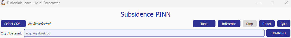
The top bar now groups every high-level control in a single row.
These buttons and fields let you load data, launch or stop a workflow, and switch between training, tuning and inference.
Select CSV… – Opens a file-chooser. Pick the .csv file containing your spatiotemporal data. The chosen filename is displayed next to the button.
Tune – Enabled as soon as a CSV (or a previous tuner manifest) is detected. Opens a setup dialog where you define the hyper-parameter search-space and the number of trials. While tuning is running the button turns orange; inference is temporarily disabled.
Inference – A toggle. It becomes active (blue) when a previously trained manifest is found next to the selected CSV. Click once to switch the GUI into inference mode (button shows orange); click again to return to training.
Stop – Appears in red once a workflow is running. Sends a graceful interruption request to the background thread (sequence generation, training, tuning or forecasting). The button is when the GUI is idle.
Reset – Clears logs, progress-bar and cached state. It also deletes the local registry cache (model checkpoints, scalers, sequence cache, …) so the next run starts from a clean slate.
Quit – Closes the application. If a workflow is active you will be asked to confirm the cancellation first.
City / Dataset – A free-text field used to name the current run (e.g. “Agnibilekrou”). The value becomes part of the output-directory path so consecutive runs never overwrite each other.
Run / Infer – Located under the log panel.
In training mode the button reads Run and launches the full end-to-end pipeline.
In inference mode it changes to Infer and only executes the prediction pipeline with the existing model.
The Run (or Infer) button is disabled while any background workflow is active; Stop and Reset reflect the opposite state.
2. Data Preview and Editing
After a CSV file is selected, a new “Preview & Edit Data” button will appear. Clicking this opens a data preview window, allowing you to perform basic cleaning and preparation steps directly within the GUI before running the main workflow.

The data editor allows for quick modifications to the loaded dataset.
This window provides several useful tools:
Table Preview: Displays the first several rows of your dataset, allowing you to verify that it was loaded correctly.
Delete row(s): Allows you to select and remove specific rows from the dataset.
Delete col(s): Allows you to select and remove unwanted columns.
Rename column: Provides a dialog to rename a selected column.
Save / Apply: Saves all changes you’ve made and closes the window, updating the dataset that will be used by the main workflow.
Cancel: Closes the window without saving any changes.
3. Model Configuration
This panel allows you to configure the model’s core architecture.
Architecture: Choose between
TransFlowSubsNet(the advanced, coupled-physics model) andPIHALNet(the consolidation-focused model).Epochs: Sets the maximum number of training epochs.
Batch Size: Defines the number of samples processed in each batch during training.
Learning Rate: Sets the initial learning rate for the Adam optimizer.
Model Type: Sets the internal data handling mode, typically ‘pihal’ or ‘tft’.
Attention Levels: A comma-separated list defining which attention mechanisms to use (e.g., ‘1, 2, 3’).
Evaluate Coverage: A checkbox to enable the calculation of quantile coverage score after prediction.
4. Training Parameters
This panel controls the temporal aspects of the training and forecasting process.
Train End Year: The last year of data to be included in the training set.
Forecast Start Year: The first year for which predictions will be made.
Forecast Horizon (Years): The number of years to predict into the future.
Time Steps (look-back): The number of historical time steps to use as input for the model’s encoder.
Quantiles (comma-separated): A list of quantiles for probabilistic forecasting (e.g., 0.1, 0.5, 0.9). Leave blank for point forecasting.
Checkpoint Format: Select the file format used when saving model checkpoints—
weights(recommended for the GUI),keras, ortf.
5. Physical Parameters
This panel gives you fine-grained control over the physics-informed components.
Pinn Coeff C, K, Ss, Q: For each physical parameter, you can select
learnableto have the model infer its value, or provide a fixed numerical value.λ Consolidation / λ GW Flow: Sets the weights (\(\lambda_c\), \(\lambda_{gw}\)) for the physics loss terms.
PDE Mode: Controls which physics constraints are active during training (e.g., ‘both’, ‘consolidation’).
Weights (Subs. / GWL): Sets the relative importance of the data-fidelity loss for the two main targets (subsidence and groundwater level).
6. Feature Selection
This panel allows you to specify which columns from your input data should be used for the different feature streams.
Dyn. / Stat. / Future: Enter the names of your columns, separated by commas, into the appropriate fields for Dynamic, Static, and Future features. Leaving a field as
autowill let the application attempt to automatically detect the appropriate columns.
7. Log and Output Panel
The large text area at the bottom of the window is the Log Panel. This is your primary window into the workflow’s progress. It provides real-time, timestamped feedback for each major step, from data loading to model training and final visualization. Any warnings or errors that occur during the process will be printed here, providing crucial information for debugging.
Once the workflow is complete, this panel will also display the head of the final results DataFrame and any generated plots, giving you an immediate preview of the outcome.
8. Viewing the Results
Once the workflow finishes successfully, the GUI provides the results in two main ways: status updates on the main window and an interactive plot viewer.
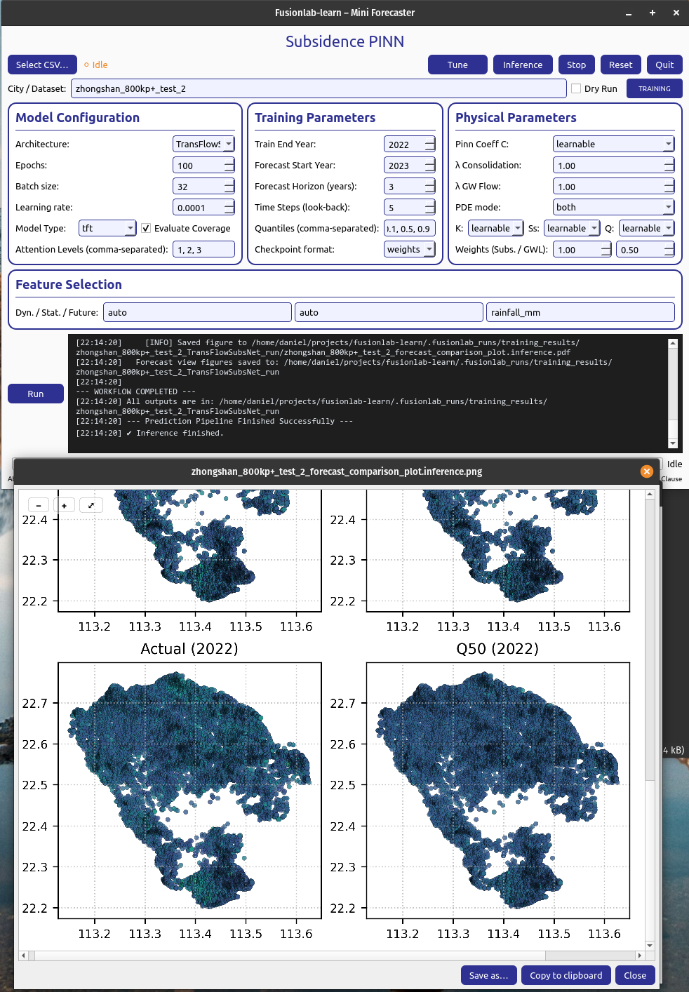

Main Window Updates (a): A checkmark and “Forecast finished” message appear at the top.If the “Evaluate Coverage” checkbox in the Model Configuration panel was ticked, the calculated coverage score (e.g., cov-result: 0.792) will be displayed in the bottom status bar.
Interactive Plot Viewer (b): A new window opens to display all plots generated during the run, such as the training history and forecast visualizations. This viewer allows you to inspect the visuals closely and provides options to “Save as…” or “Copy to clipboard” for easy export.
Zoom & Pan Controls: The viewer includes a translucent floating toolbar in the upper-left corner with “+” (zoom in), “–” (zoom out) and “□” (fit view) buttons. You can also scroll the mouse wheel to zoom and drag with the left mouse button to pan the image for detailed inspection.
Final Log Messages: The log panel will show the final messages, including confirmation that all figures have been saved and the path to the final output directory.
9. Saving Results and Artifacts
Upon successful completion of a run, the application automatically saves all generated artifacts and plots to a dedicated output directory. This ensures that your configuration, processed data, trained model, and results are preserved for later analysis and reproducibility.
The output directory is structured using the parameters from your
configuration: .fusionlab_runs/training_results/<city_name>_<model_name>_run/
Inside this directory, you will find:
Processed Data: Intermediate CSV files from the preprocessing steps.
Fitted Scalers: The saved scikit-learn scalers and encoders as .joblib files.
Trained Model: The best model checkpoint saved in the .keras format.
Forecast DataFrame: The final prediction results in a .csv file.
Visualizations: All generated plots (e.g., training history, forecast maps) saved as .png and .pdf files.
Coverage Results: If
Evaluate Coverageis enabled, the coverage score results will also be included in the output.
Running Inference with a Trained Model
The GUI is not just for training; it’s also a tool for running inference. This allows you to take a model you have already trained and apply it to a new, unseen dataset to generate predictions.
The inference workflow is automatically enabled when the application detects that a model has already been trained.
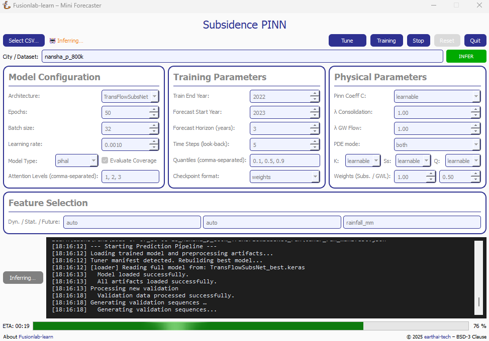
After a training run is found, the “Inference” button becomes active, allowing you to run predictions with the trained model.
How it Works:
Automatic Detection: When you select a CSV file using the “Select CSV…” button, the application automatically searches the surrounding directories trained or tuning model manifest file. This file, created at the end of a successful training run, contains all the information about the trained model and its artifacts.
Enabling the “Inference” Button: If a manifest file is found, the “Inference” button at the top right of the window will become active and turn blue, as shown in the screenshot above. Its tooltip will confirm that a trained model has been detected.
Launching the Inference Workflow:
Click the “Inference” button.
You will be prompted to select a new CSV file containing the data you want to run predictions on. This should be a file with the same structure as your original training data.
The application will then use the
PredictionPipelineto:Load the pre-trained model and its specific scalers/encoders.
Process your new data using these loaded artifacts.
Generate a forecast.
Display the results and visualizations in the output panel.
This workflow provides a seamless way to apply your trained models to new data without having to re-run the entire training process.
Hyper-parameter Tuning with the Tune Wizard
Clicking Tune opens a dedicated window that lets you define the Keras-Tuner search-space and launch a full hyper-parameter search without writing code. The wizard offers two entry points:
Easy Setup – a minimal form for non-experts: pick an algorithm, the number of trials and paste a small Python-dict with the search space.
Developer – a multi-tab notebook that exposes all knobs of the PINN models (model topology, physics weights, system settings, search limits, etc.). Each field can be fixed or declared “searchable” (e.g.
hp.Int('batch_size', 16, 128, step=16)).
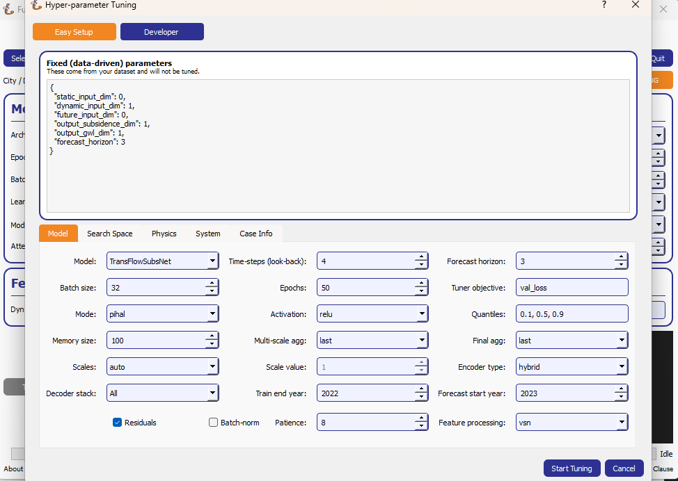
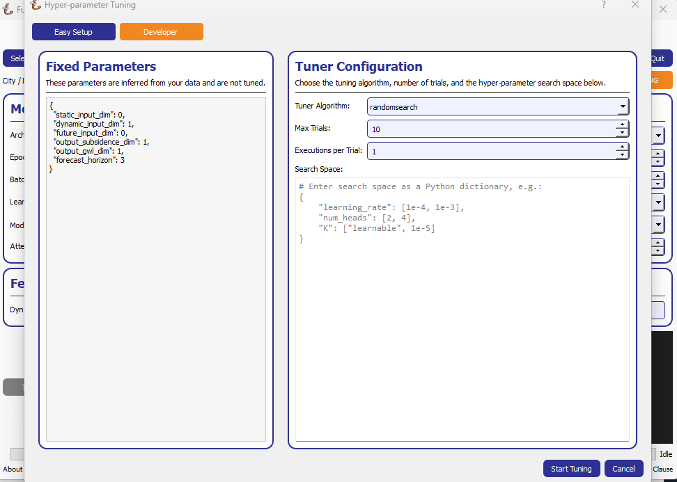
1. Wizard Workflow
The left-hand panel shows Fixed Parameters – dimensions and constants inferred from your dataset; they are not tunable.
Fill in or edit the search-space:
Developer – type a plain Python
dictsuch as:{ "learning_rate": [1e-4, 1e-3], "num_heads": [2, 4], "K": ["learnable", 1e-5] }
Easy Setup – open Search Space and click the tab next to any field to turn it into a Keras-Tuner definition (
hp.Int,hp.Float,hp.Choice…).
Choose the tuner algorithm (
randomsearch,bayesian,hyperband…), set Max Trials and Executions per Trial.Press Start Tuning. The Tune button in the main window turns orange and inference is disabled until all trials finish. The global progress-bar shows “Trial x/N – Epoch y/M – ETA”.
When the search completes, the wizard writes:
(configuration + best HPs),
<model>_best.kerasor.weights.h5, andbest_hyperparameters.json
to the run directory and re-enables inference so you can immediately test the tuned model.
The wizard therefore provides a guided, GUI-driven alternative to the
Python-level HydroTuner API – perfect for users who prefer point-and-click
experimentation.
2. Tuning in Progress
Once the Start Tuning button is pressed, the GUI enters tuning mode, as shown in the figure below. During this phase, the system executes a series of hyper-parameter trials using the configuration defined in the Tune Wizard. The main window dynamically reflects the current state of training and tuning progress.
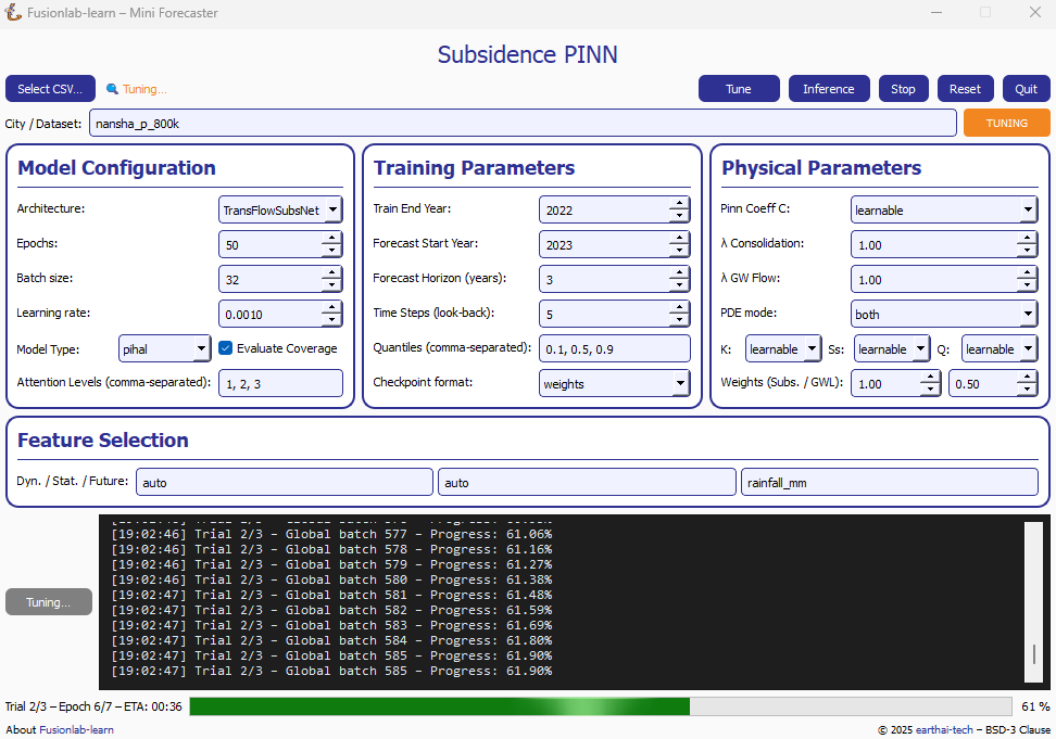
The application during an active tuning run, showing the console logs, progress bar, and disabled controls to prevent interference.
Key Elements During Tuning
Tuning Indicator: The top-right corner shows a glowing orange TUNING badge, replacing the Tune button label. This visually indicates that tuning is currently active and other operations like inference are temporarily disabled.
Live Logging Console: The central black terminal pane provides real-time updates of each trial’s progress. For instance:
Trial 2/3 – Global batch 517 – Progress: 54.18%
Trial 2/3 – Global batch 520 – Progress: 55.03%
ETA Display: A real-time ETA estimate is shown below the console to help anticipate when the current trial or tuning session will finish:
Trial 2/3 – Epoch 5/7 – ETA: 00:42
Progress Bar: A green bar at the bottom visually represents total completion, updated incrementally as tuning proceeds.
Parameter Locking: All input fields in the configuration area (e.g., model type, training parameters, physical constraints) are disabled to preserve trial consistency.
Trial Tracker: The console output shows the current trial and batch number, giving fine-grained visibility into the internal training loop during each trial.
Note
You may press Stop to interrupt the search. If so, partial results (completed trials) will still be saved to the run directory.
3. Output Files After Completion
When tuning concludes, the following files are written to disk:
best_hyperparameters.json– best trial configuration.<model>_best.kerasor.weights.h5– saved weights of the optimal model.
These can be reloaded directly for further evaluation or inference without re-running the full tuning process.