Advanced Forecasting with XTFT

This example demonstrates using the more advanced XTFT model for a multi-step quantile forecasting task. XTFT is designed to handle complex scenarios involving static features (e.g., item ID, location attributes), dynamic historical features (e.g., past sales, sensor readings), and known future inputs (e.g., planned promotions, future calendar events).

We will walk through the process step-by-step:

1. Generate synthetic multi-variate time series data for multiple items.

2. Define static, dynamic, future, and target features.

3. Scale numerical features.

4. Use the reshape_xtft_data() utility to prepare sequences suitable for XTFT.

5. Split the data into training and validation sets.

6. Define and compile an XTFT model with quantile outputs.

7. Train the model.

8. Make predictions and inverse transform them.

9. Visualize the quantile predictions for a sample item.

Prerequisites

Ensure you have fusionlab-learn and its dependencies installed:

pip install fusionlab-learn matplotlib scikit-learn joblib

Step 1: Imports and Setup

First, we import the necessary libraries, including TensorFlow, Pandas, NumPy, scikit-learn for scaling, Matplotlib for plotting, and the required components from fusionlab. We also suppress common warnings and logs for cleaner output.

import numpy as np
import pandas as pd
import tensorflow as tf
import matplotlib.pyplot as plt
from sklearn.model_selection import train_test_split
from sklearn.preprocessing import StandardScaler
import os
import joblib # For saving/loading scalers

# FusionLab imports
from fusionlab.nn.transformers import XTFT
from fusionlab.nn.utils import reshape_xtft_data
from fusionlab.nn.losses import combined_quantile_loss

# Suppress warnings and TF logs for cleaner output
import warnings
warnings.filterwarnings('ignore')
tf.get_logger().setLevel('ERROR')
if hasattr(tf, 'autograph'): # Check for autograph availability
    tf.autograph.set_verbosity(0)

# Configuration for outputs
output_dir_xtft = "./xtft_advanced_example_output"
os.makedirs(output_dir_xtft, exist_ok=True)

print("Libraries imported and TensorFlow logs configured.")

Step 2: Generate Synthetic Data

We create a sample dataset simulating monthly sales for multiple items over several years. This dataset includes static features (ItemID), dynamic features (Month, Temperature, PrevMonthSales), known future features (PlannedPromotion), and the target (Sales).

n_items = 3
n_timesteps = 36 # 3 years of monthly data
rng_seed = 42
np.random.seed(rng_seed) # For reproducibility

date_rng = pd.date_range(
    start='2020-01-01', periods=n_timesteps, freq='MS' # Month Start
    )
df_list = []

for item_id in range(n_items):
    time_idx = np.arange(n_timesteps)
    # Base sales with trend, seasonality, and item-specific factor
    sales = (
        100 + item_id * 50 + time_idx * (2 + item_id * 0.5) +
        20 * np.sin(2 * np.pi * time_idx / 12) + # Yearly seasonality
        np.random.normal(0, 10, n_timesteps) # Noise
    )
    # Simulated temperature (dynamic)
    temp = (15 + 10 * np.sin(2 * np.pi * (time_idx % 12) / 12 + np.pi) +
            np.random.normal(0, 2, n_timesteps))
    # Simulated planned promotion (future known)
    promo = np.random.randint(0, 2, n_timesteps)

    item_df = pd.DataFrame({
        'Date': date_rng,
        'ItemID': f'item_{item_id}', # String ItemID for grouping
        'Month': date_rng.month,     # Can be dynamic & future
        'Temperature': temp,
        'PlannedPromotion': promo,
        'Sales': sales
    })
    # Create lagged sales (dynamic history)
    item_df['PrevMonthSales'] = item_df['Sales'].shift(1)
    df_list.append(item_df)

df_raw = pd.concat(df_list).dropna().reset_index(drop=True)
print(f"Generated raw data shape: {df_raw.shape}")
print("Sample of generated data:")
print(df_raw.head())

Step 3: Define Features and Scale Numerics

We explicitly define which columns correspond to static, dynamic past, known future, and target roles. Numerical features are scaled using StandardScaler. The scaler for the target variable is stored for later inverse transformation of predictions.

target_col = 'Sales'
dt_col = 'Date' # Datetime column for reshaping
# ItemID is the primary static identifier for grouping
static_cols = ['ItemID']
# Dynamic features: Month, Temperature, and lagged sales
dynamic_cols = ['Month', 'Temperature', 'PrevMonthSales']
# Future features: Planned promotions and Month (known ahead)
future_cols = ['PlannedPromotion', 'Month']
# Column for grouping sequences by item
spatial_cols = ['ItemID']

# Scale numerical features (excluding ItemID, Month, PlannedPromotion)
# Target 'Sales' is also scaled.
scalers = {} # To store scalers for different columns
num_cols_to_scale = ['Temperature', 'PrevMonthSales', 'Sales']

df_scaled = df_raw.copy()
for col in num_cols_to_scale:
    if col in df_scaled.columns:
        scaler = StandardScaler()
        df_scaled[col] = scaler.fit_transform(df_scaled[[col]])
        scalers[col] = scaler # Store the fitted scaler
        print(f"Scaled column: {col}")
    else:
        print(f"Warning: Column '{col}' not found for scaling.")

# Save scalers (important for inference)
scalers_path = os.path.join(output_dir_xtft, "xtft_scalers.joblib")
joblib.dump(scalers, scalers_path)
print(f"\nScalers saved to {scalers_path}")

Step 4: Prepare Sequences using reshape_xtft_data

The reshape_xtft_data() utility transforms the processed DataFrame into the specific input arrays required by XTFT. It creates rolling windows, groups by spatial_cols (ItemID), and separates features into static, dynamic, future, and target arrays.

time_steps = 12         # Use 1 year of history as lookback
forecast_horizons = 6   # Predict next 6 months

# Note: 'ItemID' (string) needs to be numerically encoded if used
# directly as a feature by the model's embedding layers.
# For reshape_xtft_data, it's used for grouping. If also a static
# feature, ensure it's numerical or handle encoding before this step.
# Here, we assume the model's VSN/Embedding can handle integer IDs if
# 'ItemID' was label encoded and passed in static_cols.
# For simplicity, we'll assume ItemID is handled by grouping and not
# directly as a numerical static feature in this step, unless label encoded.
# If ItemID is to be a feature, it should be label encoded first.
# For this example, we'll use a placeholder if ItemID is not numeric.
# A more robust approach would be to LabelEncode 'ItemID' before this.

# Let's ensure static_cols passed to reshape_xtft_data are numeric
# If ItemID is the only static col and it's string, pass empty list or encoded.
# For this example, let's assume no additional static *features* besides grouping.
# If you had other numerical static features, list them.
processed_static_cols = [] # Example: if ItemID is only for grouping
# If ItemID were label encoded:
df_scaled['ItemID_Encoded'] = LabelEncoder().fit_transform(df_scaled['ItemID'])
processed_static_cols = ['ItemID_Encoded']

static_data, dynamic_data, future_data, target_data = reshape_xtft_data(
    df=df_scaled,
    dt_col=dt_col,
    target_col=target_col,
    dynamic_cols=dynamic_cols,
    static_cols=processed_static_cols, # Pass empty or encoded static features
    future_cols=future_cols,
    spatial_cols=spatial_cols, # Group by ItemID
    time_steps=time_steps,
    forecast_horizons=forecast_horizons,
    verbose=1 # Show resulting shapes
)
# target_data from reshape_xtft_data is (N, H, 1)

Step 5: Train/Validation Split of Sequences

The generated sequence arrays are split into training and validation sets. A simple chronological split on the sequences is used here. Inputs for the model are packaged into lists in the order [static, dynamic, future].

val_split_fraction = 0.2
# Check if any data was generated
if target_data is None or target_data.shape[0] == 0:
    raise ValueError("No sequences were generated. Check data and parameters.")

n_samples = target_data.shape[0]
split_idx = int(n_samples * (1 - val_split_fraction))

# Handle cases where static_data might be None
X_train_static = static_data[:split_idx] if static_data is not None else None
X_val_static = static_data[split_idx:] if static_data is not None else None

X_train_dynamic, X_val_dynamic = dynamic_data[:split_idx], dynamic_data[split_idx:]
X_train_future, X_val_future = future_data[:split_idx], future_data[split_idx:]
y_train, y_val = target_data[:split_idx], target_data[split_idx:]

train_inputs = [X_train_static, X_train_dynamic, X_train_future]
val_inputs = [X_val_static, X_val_dynamic, X_val_future]

print(f"\nData split into Train/Validation sequences:")
print(f"  Train samples: {len(y_train)}")
print(f"  Validation samples: {len(y_val)}")

Step 6: Define XTFT Model for Quantile Forecast

Instantiate the XTFT model. Input dimensions are derived from the prepared data arrays. Configure for quantile forecasting and set relevant XTFT hyperparameters.

quantiles_to_predict = [0.1, 0.5, 0.9]
output_dim_model = 1 # Predicting univariate 'Sales'

# Determine input dimensions for the model
s_dim = X_train_static.shape[-1] if X_train_static is not None else 0
d_dim = X_train_dynamic.shape[-1]
f_dim = X_train_future.shape[-1] if X_train_future is not None else 0

model = XTFT(
    static_input_dim=s_dim,
    dynamic_input_dim=d_dim,
    future_input_dim=f_dim,
    forecast_horizon=forecast_horizons,
    quantiles=quantiles_to_predict,
    output_dim=output_dim_model,
    # Example XTFT Hyperparameters (these should be tuned)
    embed_dim=16,
    lstm_units=32,
    attention_units=16,
    hidden_units=32,
    num_heads=2, # Reduced for speed
    dropout_rate=0.1,
    max_window_size=time_steps, # Can be different from time_steps
    memory_size=20, # Reduced for speed
    scales=[1, 3]   # Example multi-scale config
)
print("\nXTFT model instantiated for quantile forecast.")

Step 7: Compile and Train the Model

Compile the model with an Adam optimizer and the combined_quantile_loss(). Train for a few epochs for this demonstration.

loss_fn = combined_quantile_loss(quantiles=quantiles_to_predict)
model.compile(
    optimizer=tf.keras.optimizers.Adam(learning_rate=0.005),
    loss=loss_fn
    )
print("XTFT model compiled with quantile loss.")

# Dummy call to build model and print summary (optional)
# Ensure inputs are correctly structured (list of 3, Nones allowed if dims are 0)
dummy_s = tf.zeros((1, s_dim)) if s_dim > 0 else None
dummy_d = tf.zeros((1, time_steps, d_dim))
dummy_f = tf.zeros((1, time_steps + forecast_horizons, f_dim)) if f_dim > 0 else None
# model([dummy_s, dummy_d, dummy_f])
# model.summary(line_length=100)


print("\nStarting XTFT model training (few epochs for demo)...")
history = model.fit(
    train_inputs, # List [Static, Dynamic, Future]
    y_train,      # Targets
    validation_data=(val_inputs, y_val),
    epochs=5,     # Increase for real training
    batch_size=16,  # Adjust based on memory and dataset size
    verbose=1
)
print("Training finished.")
if history and history.history.get('val_loss'):
    print(f"Final validation loss: {history.history['val_loss'][-1]:.4f}")

Step 8: Make Predictions and Inverse Transform

Use the trained model to predict on the validation set. Then, inverse transform the scaled predictions and actuals back to their original units.

print("\nMaking quantile predictions on validation set...")
predictions_scaled = model.predict(val_inputs, verbose=0)
# Shape: (NumValSamples, Horizon, NumQuantiles) if output_dim=1

# Inverse Transform Predictions and Actuals
# We need the scaler for the 'Sales' (target) column
target_scaler = scalers.get(target_col)
if target_scaler is None:
    print("Warning: Target scaler not found. Plotting scaled values.")
    predictions_final = predictions_scaled
    y_val_final = y_val
else:
    num_val_samples = X_val_static.shape[0] if X_val_static is not None else X_val_dynamic.shape[0]
    num_q = len(quantiles_to_predict)

    # Reshape for scaler: (Samples*Horizon, Quantiles/OutputDim)
    pred_reshaped = predictions_scaled.reshape(-1, num_q * output_dim_model)
    # If output_dim_model > 1, inverse_transform needs care.
    # Assuming output_dim_model = 1 for simplicity here.
    if output_dim_model == 1:
        predictions_inv = target_scaler.inverse_transform(pred_reshaped)
        predictions_final = predictions_inv.reshape(
            num_val_samples, forecast_horizons, num_q
        )
        # Inverse transform actuals
        y_val_reshaped = y_val.reshape(-1, output_dim_model)
        y_val_inv = target_scaler.inverse_transform(y_val_reshaped)
        y_val_final = y_val_inv.reshape(
            num_val_samples, forecast_horizons, output_dim_model
        )
        print("Predictions and actuals inverse transformed.")
    else: # output_dim > 1, inverse transform is more complex
        print("Inverse transform for multi-output quantiles not shown, plotting scaled.")
        predictions_final = predictions_scaled
        y_val_final = y_val

Step 9: Visualize Forecast for One Item

Plot the actual sales and the predicted quantiles (median line plus shaded interval) for one sample item from the validation set.

# Select an item and its first sequence in the validation set for plotting
# This requires ItemID to be part of X_val_static if it was numerically encoded
# For simplicity, we'll plot the first validation sequence.
sample_to_plot_idx = 0

actual_vals_item = y_val_final[sample_to_plot_idx, :, 0] # Assuming output_dim=1
pred_quantiles_item = predictions_final[sample_to_plot_idx, :, :]

# Create an approximate time axis for the forecast period
# This needs the last date of the training data corresponding to this sequence
# For a generic plot, use forecast steps
forecast_steps_axis = np.arange(1, forecast_horizons + 1)

plt.figure(figsize=(12, 6))
plt.plot(forecast_steps_axis, actual_vals_item,
         label='Actual Sales', marker='o', linestyle='--')
plt.plot(forecast_steps_axis, pred_quantiles_item[:, 1], # Median (0.5 quantile)
         label='Median Forecast (q=0.5)', marker='x')
plt.fill_between(
    forecast_steps_axis,
    pred_quantiles_item[:, 0], # Lower quantile (q=0.1)
    pred_quantiles_item[:, 2], # Upper quantile (q=0.9)
    color='gray', alpha=0.3,
    label='Prediction Interval (q=0.1 to q=0.9)'
)
plt.title(f'XTFT Quantile Forecast (Validation Sample {sample_to_plot_idx})')
plt.xlabel('Forecast Step into Horizon')
plt.ylabel(f'{target_col} (Units after Inverse Transform if applied)')
plt.legend(); plt.grid(True); plt.tight_layout()
# To save the figure:
# fig_path = os.path.join(output_dir_xtft, "advanced_xtft_quantile_forecast.png")
# plt.savefig(fig_path)
# print(f"Plot saved to {fig_path}")
plt.show()
print("\nAdvanced XTFT quantile forecasting example complete.")

Example Output Plot:

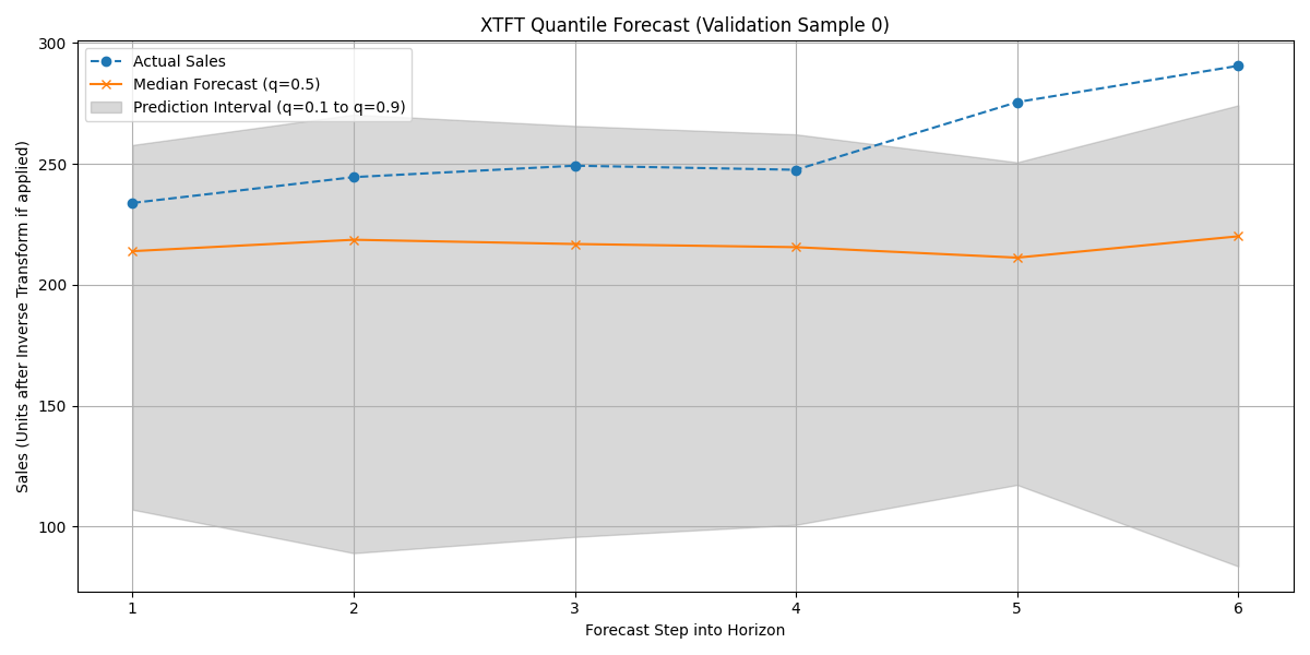
Visualization of the XTFT quantile forecast (median and interval) against actual validation data for a sample item.