Exercise: Advanced Forecasting with SuperXTFT
Welcome to this exercise on using the advanced
SuperXTFT model from fusionlab-learn.
SuperXTFT enhances the powerful XTFT
architecture by incorporating additional components, such as input
Variable Selection Networks (VSNs) and post-processing Gated
Residual Networks (GRNs), to maximize representation learning.
Note
SuperXTFT is a production-ready model and represents the most
powerful, feature-rich version in the TFT family. It is the
recommended choice when you are aiming for maximum predictive
performance and have the computational resources for a deeper, more
parameter-rich model.
Learning Objectives:
Leverage the advanced
SuperXTFTmodel for a complex forecasting task.Understand that the data preparation workflow is identical to that for
XTFT.Perform a multi-step quantile forecast to generate probabilistic predictions.
Visualize the forecast results, including their uncertainty intervals.
Let’s begin!
Prerequisites
Ensure you have fusionlab-learn and its common dependencies
installed.
pip install fusionlab-learn matplotlib scikit-learn joblib
Step 1: Imports and Setup
We start by importing necessary libraries and fusionlab components.
 1import numpy as np
 2import pandas as pd
 3import tensorflow as tf
 4import matplotlib.pyplot as plt
 5from sklearn.model_selection import train_test_split
 6from sklearn.preprocessing import StandardScaler
 7import os
 8import joblib
 9import warnings
10
11# FusionLab imports
12from fusionlab.nn.transformers import SuperXTFT
13from fusionlab.nn.utils import reshape_xtft_data
14from fusionlab.nn.losses import combined_quantile_loss
15from fusionlab.datasets.make import make_multi_feature_time_series
16
17# Suppress warnings and TF logs
18warnings.filterwarnings('ignore')
19os.environ['TF_CPP_MIN_LOG_LEVEL'] = '2'
20tf.get_logger().setLevel('ERROR')
21if hasattr(tf, 'autograph'):
22    tf.autograph.set_verbosity(0)
23
24exercise_output_dir_super_xtft = "./super_xtft_exercise_outputs"
25os.makedirs(exercise_output_dir_super_xtft, exist_ok=True)
26
27print("Libraries imported for SuperXTFT exercise.")
Expected Output 1.1:
Libraries imported for SuperXTFT exercise.
Step 2: Generate Synthetic Multi-Feature Data
We’ll use the same data generation setup as the advanced XTFT exercise, as SuperXTFT also expects static, dynamic, and future inputs.
 1n_items_sxtft = 2
 2n_timesteps_sxtft = 36 # Shorter for quicker run
 3rng_seed_sxtft = 42
 4np.random.seed(rng_seed_sxtft)
 5tf.random.set_seed(rng_seed_sxtft)
 6
 7data_bunch_sxtft = make_multi_feature_time_series(
 8    n_series=n_items_sxtft, n_timesteps=n_timesteps_sxtft,
 9    freq='MS', seasonality_period=12,
10    seed=rng_seed_sxtft, as_frame=False
11)
12df_raw_sxtft = data_bunch_sxtft.frame.copy()
13print(f"Generated raw data shape for SuperXTFT exercise: {df_raw_sxtft.shape}")
14print(df_raw_sxtft.head(3))
Expected Output 2.2:
Generated raw data shape for SuperXTFT exercise: (72, 9)
        date  series_id  base_level  ...  month  future_event     target
0 2020-01-01          0   50.049671  ...      1             1  63.055435
1 2020-02-01          0   50.049671  ...      2             1  68.394497
2 2020-03-01          0   50.049671  ...      3             1  70.075474

[3 rows x 9 columns]
Step 3: Define Feature Roles and Scale Numerical Data
We use feature lists from the data_bunch and scale numerical features. series_id is numerical and will be used as a static feature.
 1target_col_sxtft = data_bunch_sxtft.target_col
 2dt_col_sxtft = data_bunch_sxtft.dt_col
 3static_cols_sxtft = data_bunch_sxtft.static_features
 4dynamic_cols_sxtft = data_bunch_sxtft.dynamic_features
 5future_cols_sxtft = data_bunch_sxtft.future_features
 6spatial_cols_sxtft = [data_bunch_sxtft.spatial_id_col]
 7
 8scalers_sxtft = {}
 9num_cols_to_scale_sxtft = ['base_level', 'dynamic_cov',
10                           'target_lag1', target_col_sxtft]
11df_scaled_sxtft = df_raw_sxtft.copy()
12
13for col in num_cols_to_scale_sxtft:
14    if col in df_scaled_sxtft.columns and \
15       pd.api.types.is_numeric_dtype(df_scaled_sxtft[col]):
16        scaler = StandardScaler()
17        df_scaled_sxtft[col] = scaler.fit_transform(df_scaled_sxtft[[col]])
18        scalers_sxtft[col] = scaler
19print(f"\nNumerical features scaled: {num_cols_to_scale_sxtft}")
Expected Output 3.3:
Numerical features scaled: ['base_level', 'dynamic_cov', 'target_lag1', 'target']
Step 4: Prepare Sequences using reshape_xtft_data
Transform the DataFrame into structured arrays for SuperXTFT.
 1time_steps_sxtft = 12
 2forecast_horizons_sxtft = 6
 3
 4s_data_sxtft, d_data_sxtft, f_data_sxtft, t_data_sxtft = \
 5    reshape_xtft_data(
 6        df=df_scaled_sxtft, dt_col=dt_col_sxtft,
 7        target_col=target_col_sxtft,
 8        dynamic_cols=dynamic_cols_sxtft,
 9        static_cols=static_cols_sxtft, # Includes series_id, base_level
10        future_cols=future_cols_sxtft,
11        spatial_cols=spatial_cols_sxtft,
12        time_steps=time_steps_sxtft,
13        forecast_horizons=forecast_horizons_sxtft,
14        verbose=0 # Suppress reshape logs for brevity
15    )
16print(f"\nReshaped Data Shapes for SuperXTFT:")
17print(f"  Static : {s_data_sxtft.shape}")
18print(f"  Dynamic: {d_data_sxtft.shape}")
19print(f"  Future : {f_data_sxtft.shape}")
20print(f"  Target : {t_data_sxtft.shape}")
- Expected Output 4.4:
(For N_series=2, N_timesteps=36, T=12, H=6: Seq/series = 36-12-6+1 = 19. Total = 2*19 = 38)
Reshaped Data Shapes for SuperXTFT:
  Static : (38, 2)
  Dynamic: (38, 12, 4)
  Future : (38, 18, 3)
  Target : (38, 6, 1)
Step 5: Train/Validation Split of Sequences
Split sequence arrays for training and validation.
 1val_split_sxtft_frac = 0.25 # Using a bit more for validation
 2n_samples_sxtft = s_data_sxtft.shape[0]
 3split_idx_sxtft = int(n_samples_sxtft * (1 - val_split_sxtft_frac))
 4
 5X_s_train_sxtft, X_s_val_sxtft = s_data_sxtft[:split_idx_sxtft], s_data_sxtft[split_idx_sxtft:]
 6X_d_train_sxtft, X_d_val_sxtft = d_data_sxtft[:split_idx_sxtft], d_data_sxtft[split_idx_sxtft:]
 7X_f_train_sxtft, X_f_val_sxtft = f_data_sxtft[:split_idx_sxtft], f_data_sxtft[split_idx_sxtft:]
 8y_t_train_sxtft, y_t_val_sxtft = t_data_sxtft[:split_idx_sxtft], t_data_sxtft[split_idx_sxtft:]
 9
10train_inputs_sxtft = [X_s_train_sxtft, X_d_train_sxtft, X_f_train_sxtft]
11val_inputs_sxtft = [X_s_val_sxtft, X_d_val_sxtft, X_f_val_sxtft]
12
13print(f"\nData split for SuperXTFT. Train: {len(y_t_train_sxtft)}, "
14      f"Val: {len(y_t_val_sxtft)}")
Expected Output 5.5:
Data split for SuperXTFT. Train: 28, Val: 10
Step 6: Define SuperXTFT Model for Quantile Forecast
Instantiate the SuperXTFT model. Its parameters
are similar to XTFT. We’ll explicitly disable anomaly detection for
this exercise.
 1quantiles_sxtft = [0.1, 0.5, 0.9]
 2output_dim_sxtft = 1
 3
 4s_dim_sxtft = X_s_train_sxtft.shape[-1]
 5d_dim_sxtft = X_d_train_sxtft.shape[-1]
 6f_dim_sxtft = X_f_train_sxtft.shape[-1]
 7
 8super_xtft_model_ex = SuperXTFT(
 9    static_input_dim=s_dim_sxtft,
10    dynamic_input_dim=d_dim_sxtft,
11    future_input_dim=f_dim_sxtft,
12    forecast_horizon=forecast_horizons_sxtft,
13    quantiles=quantiles_sxtft,
14    output_dim=output_dim_sxtft,
15    # Minimal HPs for faster demo
16    embed_dim=8, lstm_units=16, attention_units=8,
17    hidden_units=16, num_heads=1, dropout_rate=0.0,
18    max_window_size=time_steps_sxtft, memory_size=10,
19    scales=None,
20    anomaly_detection_strategy=None, # Explicitly disable
21    anomaly_loss_weight=0.0
22)
23print("\nSuperXTFT model instantiated (anomaly detection disabled).")
Step 7: Compile and Train the SuperXTFT Model
Compile with quantile loss and train for a few epochs.
 1loss_fn_sxtft = combined_quantile_loss(quantiles=quantiles_sxtft)
 2super_xtft_model_ex.compile(
 3    optimizer=tf.keras.optimizers.Adam(learning_rate=0.005),
 4    loss=loss_fn_sxtft
 5    )
 6print("SuperXTFT model compiled.")
 7
 8# Optional: Build model with dummy inputs to print summary
 9# try:
10#     dummy_s = tf.zeros((1, s_dim_sxtft))
11#     dummy_d = tf.zeros((1, time_steps_sxtft, d_dim_sxtft))
12#     dummy_f = tf.zeros((1, time_steps_sxtft + forecast_horizons_sxtft, f_dim_sxtft))
13#     super_xtft_model_ex([dummy_s, dummy_d, dummy_f])
14#     super_xtft_model_ex.summary(line_length=90)
15# except Exception as e:
16#     print(f"Model build/summary error: {e}")
17
18print("\nStarting SuperXTFT model training...")
19history_sxtft = super_xtft_model_ex.fit(
20    train_inputs_sxtft, y_t_train_sxtft,
21    validation_data=(val_inputs_sxtft, y_t_val_sxtft),
22    epochs=3, batch_size=4, verbose=1 # Short run for demo
23)
24print("SuperXTFT Training finished.")
25if history_sxtft and history_sxtft.history.get('val_loss'):
26    val_loss_sxtft = history_sxtft.history['val_loss'][-1]
27    print(f"Final validation loss: {val_loss_sxtft:.4f}")
- Expected Output 7.7:
(Keras training logs and final validation loss)
SuperXTFT model compiled.

Starting SuperXTFT model training...
Epoch 1/3
7/7 [==============================] - 17s 329ms/step - loss: 0.4341 - val_loss: 0.5377
Epoch 2/3
7/7 [==============================] - 0s 12ms/step - loss: 0.4233 - val_loss: 0.5354
Epoch 3/3
7/7 [==============================] - 0s 12ms/step - loss: 0.4135 - val_loss: 0.5387
SuperXTFT Training finished.
Final validation loss: 0.5387
Step 8: Make Predictions and Visualize
Predict on the validation set and visualize the quantile forecast for a sample item, similar to the XTFT example.
 1print("\nMaking quantile predictions with SuperXTFT...")
 2val_pred_scaled_sxtft = super_xtft_model_ex.predict(
 3    val_inputs_sxtft, verbose=0
 4    )
 5print(f"Scaled prediction output shape: {val_pred_scaled_sxtft.shape}")
 6
 7# Inverse Transform (simplified, assumes target was scaled)
 8target_scaler_sxtft = scalers_sxtft.get(target_col_sxtft)
 9if target_scaler_sxtft:
10    num_val_sxtft = X_s_val_sxtft.shape[0]
11    num_q_sxtft = len(quantiles_sxtft)
12
13    pred_flat_sxtft = val_pred_scaled_sxtft.reshape(-1, num_q_sxtft)
14    actual_flat_sxtft = y_t_val_sxtft.reshape(-1, 1)
15
16    pred_inv_sxtft = target_scaler_sxtft.inverse_transform(pred_flat_sxtft)
17    actual_inv_sxtft = target_scaler_sxtft.inverse_transform(actual_flat_sxtft)
18
19    pred_final_sxtft = pred_inv_sxtft.reshape(val_pred_scaled_sxtft.shape)
20    actual_final_sxtft = actual_inv_sxtft.reshape(y_t_val_sxtft.shape)
21    print("Predictions and actuals inverse transformed.")
22else:
23    print("Warning: Target scaler not found. Plotting scaled values.")
24    pred_final_sxtft = val_pred_scaled_sxtft
25    actual_final_sxtft = y_t_val_sxtft
26
27# --- Visualization for one sample item ---
28sample_idx_sxtft = 0 # Plot the first validation sequence
29if len(actual_final_sxtft) > sample_idx_sxtft:
30    actual_sxtft_item = actual_final_sxtft[sample_idx_sxtft, :, 0]
31    pred_q_sxtft_item = pred_final_sxtft[sample_idx_sxtft, :, :]
32    steps_axis_sxtft = np.arange(1, forecast_horizons_sxtft + 1)
33
34    plt.figure(figsize=(12, 6))
35    plt.plot(steps_axis_sxtft, actual_sxtft_item,
36             label='Actual Sales', marker='o', linestyle='--')
37    plt.plot(steps_axis_sxtft, pred_q_sxtft_item[:, 1], # Median
38             label='Median Forecast (q=0.5)', marker='x')
39    plt.fill_between(
40        steps_axis_sxtft, pred_q_sxtft_item[:, 0], pred_q_sxtft_item[:, 2],
41        color='lightcoral', alpha=0.4,
42        label='Interval (q0.1-q0.9)'
43    )
44    plt.title(f'SuperXTFT Quantile Forecast (Sample {sample_idx_sxtft})')
45    plt.xlabel('Forecast Step'); plt.ylabel(target_col_sxtft)
46    plt.legend(); plt.grid(True); plt.tight_layout()
47    # fig_path_sxtft = os.path.join(
48    # exercise_output_dir_super_xtft,
49    # "exercise_super_xtft_forecast.png")
50    # plt.savefig(fig_path_sxtft)
51    plt.show()
52    print("\nSuperXTFT quantile forecast plot generated.")
53else:
54    print("\nNot enough validation samples to plot.")
Expected Plot 8.8:
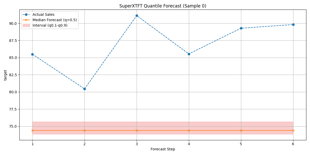
Visualization of the SuperXTFT quantile forecast (median and interval) against actual validation data.
Discussion of Exercise
Congratulations! You have successfully completed the end-to-end
workflow for using the advanced SuperXTFT model.
This exercise has demonstrated several key points:
The data preparation steps (feature definition, scaling, and sequence generation) are identical to those for the standard
XTFTmodel. This makes it easy to upgrade your workflow to use this more powerful architecture without changing your data pipeline.Instantiation and compilation follow the same familiar pattern, using a consistent set of core hyperparameters.
The key enhancements of
SuperXTFT—its input Variable Selection Networks for feature selection and its post-attention Gated Residual Networks for deeper processing—are seamlessly integrated within its internal architecture. This allows you to leverage its additional power without altering your core training and prediction code.
You have successfully trained the most powerful model in the fusionlab-learn
TFT family. For new projects, it is often a good strategy to start
with the standard XTFT as a robust baseline, and
then upgrade to SuperXTFT when you need to push for the highest
possible performance, especially on datasets with many features or
complex underlying dynamics.