Exercise: Quantile Forecasting with TFT Variants

Welcome to this exercise on quantile forecasting! Quantile forecasts provide an estimate of the prediction uncertainty by predicting multiple quantiles (e.g., 10th, 50th, 90th percentiles) instead of a single point value. This is crucial for understanding the range of potential future outcomes.

In this guide, you’ll learn to use two Temporal Fusion Transformer variants from fusionlab-learn for this task: 1. The flexible TemporalFusionTransformer. 2. The stricter TFT.

Learning Objectives:

• Prepare data for multi-step quantile forecasting.

• Instantiate and compile TFT models for quantile outputs using the quantiles parameter and combined_quantile_loss().

• Correctly format inputs for both flexible (optional inputs) and stricter (all inputs required) TFT variants.

• Train the models and interpret their multi-quantile predictions.

• Visualize quantile forecasts to represent prediction uncertainty.

Let’s begin!

Prerequisites

Ensure you have fusionlab-learn and its common dependencies installed. For visualizations, matplotlib is also needed.

pip install fusionlab-learn matplotlib scikit-learn joblib

Exercise 1: Quantile Forecasting with Flexible TemporalFusionTransformer

In this part, we’ll use the flexible TemporalFusionTransformer with only dynamic (past observed) features to produce multi-step quantile forecasts.

Workflow: 1. Generate synthetic time series data. 2. Prepare sequences for multi-step forecasting. 3. Define and compile the flexible TFT for quantile output. 4. Train the model. 5. Make and visualize quantile predictions.

Step 1.1: Imports and Setup

Import necessary libraries and fusionlab components.

import numpy as np
import pandas as pd
import tensorflow as tf
import matplotlib.pyplot as plt
import warnings
import os

# FusionLab imports
from fusionlab.nn.transformers import TemporalFusionTransformer
from fusionlab.nn.utils import create_sequences
from fusionlab.nn.losses import combined_quantile_loss
# for preparing dummy tensor when static and future are None
from fusionlab.nn.utils import prepare_model_inputs

# Suppress warnings and TF logs
warnings.filterwarnings('ignore')
tf.get_logger().setLevel('ERROR')
if hasattr(tf, 'autograph'):
    tf.autograph.set_verbosity(0)

# Directory for saving outputs
exercise_output_dir_quant = "./quantile_forecast_exercise_outputs"
os.makedirs(exercise_output_dir_quant, exist_ok=True)

print("Libraries imported for Flexible TFT Quantile Exercise.")

Expected Output 1.1:

Libraries imported for Flexible TFT Quantile Exercise.

Step 1.2: Generate Synthetic Data

We use a simple sine wave with noise.

np.random.seed(42) # For reproducibility
tf.random.set_seed(42)

time_flex_q = np.arange(0, 100, 0.1)
amplitude_flex_q = np.sin(time_flex_q) + \
                   np.random.normal(0, 0.15, len(time_flex_q))
df_flex_q = pd.DataFrame({'Value': amplitude_flex_q})
print(f"Generated data shape for flexible TFT: {df_flex_q.shape}")

Expected Output 1.2:

Generated data shape for flexible TFT: (1000, 1)

Step 1.3: Prepare Sequences for Multi-Step Forecasting

We’ll predict the next 5 time steps using the past 10 steps. Targets are reshaped to (Samples, Horizon, OutputDim).

sequence_length_flex_q = 10
forecast_horizon_flex_q = 5 # Predict next 5 steps
target_col_flex_q = 'Value'

sequences_flex_q, targets_flex_q = create_sequences(
    df=df_flex_q,
    sequence_length=sequence_length_flex_q,
    target_col=target_col_flex_q,
    forecast_horizon=forecast_horizon_flex_q,
    verbose=0
)
sequences_flex_q = sequences_flex_q.astype(np.float32)
targets_flex_q = targets_flex_q.reshape(
    -1, forecast_horizon_flex_q, 1 # OutputDim = 1
    ).astype(np.float32)

print(f"\nFlexible TFT - Input sequences (X): {sequences_flex_q.shape}")
print(f"Flexible TFT - Target values (y): {targets_flex_q.shape}")

Expected Output 1.3:

(Num samples = 1000 - 10 - 5 + 1 = 986)

Flexible TFT - Input sequences (X): (986, 10, 1)
Flexible TFT - Target values (y): (986, 5, 1)

Step 1.4: Define Flexible TFT Model for Quantile Forecast

Instantiate TemporalFusionTransformer, providing the quantiles list. Static and future input dimensions default to None.

quantiles_to_predict_flex = [0.1, 0.5, 0.9] # 10th, 50th, 90th
num_dynamic_features_flex_q = sequences_flex_q.shape[-1]

model_flex_q = TemporalFusionTransformer(
    dynamic_input_dim=num_dynamic_features_flex_q,
    forecast_horizon=forecast_horizon_flex_q,
    output_dim=1, # Univariate target
    hidden_units=16, num_heads=2,
    num_lstm_layers=1, lstm_units=16,
    quantiles=quantiles_to_predict_flex # Enable quantile output
)
print("\nFlexible TFT for quantiles instantiated.")

# Compile with combined_quantile_loss
loss_fn_flex_q = combined_quantile_loss(
    quantiles=quantiles_to_predict_flex
    )
model_flex_q.compile(optimizer='adam', loss=loss_fn_flex_q)
print("Flexible TFT compiled with quantile loss.")

Expected Output 1.4:

Flexible TFT for quantiles instantiated.
Flexible TFT compiled with quantile loss.

Step 1.5: Train the Model

Inputs are passed as [None, dynamic_sequences, None] for the [static, dynamic, future] order.

# Preparing dummy tensor or pass only to the model [sequences_flex_q]
train_inputs_flex_q = prepare_model_inputs(
    dynamic_input=sequences_flex_q,
     static_input=None, future_input=None,
     model_type= 'strict')

# train_inputs_flex_q  Order: [Static, Dynamic, Future]
# Try also : train_inputs_flex_q =[sequences_flex_q]
print("\nStarting flexible TFT training (quantile)...")
history_flex_q = model_flex_q.fit(
    train_inputs_flex_q,
    targets_flex_q, # Shape (Samples, Horizon, 1)
    epochs=10,      # Train a bit longer for quantiles
    batch_size=32,
    validation_split=0.2,
    verbose=1       # Show progress
)
print("Flexible TFT training finished.")
if history_flex_q and history_flex_q.history.get('val_loss'):
    val_loss_q = history_flex_q.history['val_loss'][-1]
    print(f"Final validation loss (quantile): {val_loss_q:.4f}")

Expected Output 1.5:

(Keras training logs for 10 epochs, then final loss: loss may varie)

Starting flexible TFT training (quantile)...
Epoch 1/10
25/25 [==============================] - 7s 47ms/step - loss: 0.2302 - val_loss: 0.1550
Epoch 2/10
25/25 [==============================] - 0s 8ms/step - loss: 0.1629 - val_loss: 0.1312
Epoch 3/10
25/25 [==============================] - 0s 9ms/step - loss: 0.1470 - val_loss: 0.1179
Epoch 4/10
25/25 [==============================] - 0s 9ms/step - loss: 0.1354 - val_loss: 0.1136
Epoch 5/10
25/25 [==============================] - 0s 9ms/step - loss: 0.1278 - val_loss: 0.1080
Epoch 6/10
25/25 [==============================] - 0s 8ms/step - loss: 0.1255 - val_loss: 0.1071
Epoch 7/10
25/25 [==============================] - 0s 9ms/step - loss: 0.1212 - val_loss: 0.1019
Epoch 8/10
25/25 [==============================] - 0s 9ms/step - loss: 0.1161 - val_loss: 0.1003
Epoch 9/10
25/25 [==============================] - 0s 8ms/step - loss: 0.1113 - val_loss: 0.0974
Epoch 10/10
25/25 [==============================] - 0s 8ms/step - loss: 0.1060 - val_loss: 0.0890
Flexible TFT training finished.
Final validation loss (quantile): 0.0890

Step 1.6: Make and Visualize Quantile Predictions

Predictions will have a shape (Batch, Horizon, NumQuantiles). We visualize the median and the prediction interval.

num_samples_total_flex_q = sequences_flex_q.shape[0]
val_start_idx_flex_q = int(num_samples_total_flex_q * (1 - 0.2))

val_dynamic_flex_q = sequences_flex_q[val_start_idx_flex_q:]
val_actuals_flex_q = targets_flex_q[val_start_idx_flex_q:]

val_inputs_list_flex_q = [val_dynamic_flex_q]

print("\nMaking quantile predictions (flexible TFT)...")
val_predictions_flex_q = model_flex_q.predict(
    val_inputs_list_flex_q, verbose=0
    )
print(f"Prediction output shape: {val_predictions_flex_q.shape}")

# --- Visualization for one sample ---
sample_to_plot_flex_q = 0 # Plot the first sample from validation
actual_vals_plot_flex = val_actuals_flex_q[sample_to_plot_flex_q, :, 0]
pred_quantiles_plot_flex = val_predictions_flex_q[sample_to_plot_flex_q, :, :]

# Align time axis for plotting
plot_time_flex_q = time_flex_q[
    val_start_idx_flex_q + sequence_length_flex_q + sample_to_plot_flex_q : \
    val_start_idx_flex_q + sequence_length_flex_q + \
        sample_to_plot_flex_q + forecast_horizon_flex_q
    ]

plt.figure(figsize=(12, 6))
plt.plot(plot_time_flex_q, actual_vals_plot_flex,
         label='Actual Value', marker='o', linestyle='--')
plt.plot(plot_time_flex_q, pred_quantiles_plot_flex[:, 1], # Median (0.5)
         label='Predicted Median (q=0.5)', marker='x')
plt.fill_between(
    plot_time_flex_q,
    pred_quantiles_plot_flex[:, 0], # Lower quantile (q=0.1)
    pred_quantiles_plot_flex[:, 2], # Upper quantile (q=0.9)
    color='skyblue', alpha=0.4,
    label='Prediction Interval (q0.1-q0.9)'
)
plt.title('Flexible TFT Quantile Forecast (Dynamic Inputs Only)')
plt.xlabel('Time'); plt.ylabel('Value')
plt.legend(); plt.grid(True); plt.tight_layout()
# To save for documentation:
# plt.savefig(os.path.join(exercise_output_dir_quant,
#                          "exercise_quantile_tft_flexible.png"))
plt.show()
print("Flexible TFT quantile plot generated.")

Expected Plot 1.6:

Visualization of the quantile forecast (median and interval) against actual validation data using the flexible TemporalFusionTransformer.

---

Exercise 2: Quantile Forecasting with Stricter TFT

Now, we use the stricter TFT class, which requires static, dynamic, and future inputs.

Workflow: 1. Generate synthetic data with all three feature types. 2. Define feature roles, encode categoricals, and scale numerics. 3. Use reshape_xtft_data() to prepare

the three distinct input arrays.

4. Define and compile the stricter TFT for quantile output.

5. Train the model.

6. Make and visualize quantile predictions.

Step 2.1: Imports for Stricter TFT

(Most imports are already done. We might need LabelEncoder.)

from sklearn.preprocessing import LabelEncoder # For ItemID
from fusionlab.datasets.make import make_multi_feature_time_series
from fusionlab.nn.transformers import TFT as TFTStricter # Alias
from fusionlab.nn.utils import reshape_xtft_data

print("\nLibraries ready for Stricter TFT Quantile Exercise.")

Step 2.2: Generate Synthetic Multi-Feature Data

We use make_multi_feature_time_series for convenience.

n_items_strict_q = 2
n_timesteps_strict_q = 60
rng_seed_strict_q = 123
np.random.seed(rng_seed_strict_q)
tf.random.set_seed(rng_seed_strict_q)

data_bunch_strict_q = make_multi_feature_time_series(
    n_series=n_items_strict_q,
    n_timesteps=n_timesteps_strict_q,
    freq='D', seasonality_period=7, seed=rng_seed_strict_q,
    as_frame=False # Get Bunch object
)
df_raw_strict_q = data_bunch_strict_q.frame.copy()
print(f"\nGenerated data for stricter TFT: {df_raw_strict_q.shape}")

Expected Output 2.2:

Generated data for stricter TFT: (120, 9)

Step 2.3: Define Features, Encode, and Scale

We use feature lists from data_bunch_strict_q. series_id (our ItemID) is numerical from the data generator. Numerical features are scaled.

target_col_sq = data_bunch_strict_q.target_col
dt_col_sq = data_bunch_strict_q.dt_col
static_cols_sq = data_bunch_strict_q.static_features
dynamic_cols_sq = data_bunch_strict_q.dynamic_features
future_cols_sq = data_bunch_strict_q.future_features
spatial_cols_sq = [data_bunch_strict_q.spatial_id_col]

df_processed_sq = df_raw_strict_q.copy()
scalers_sq = {}
num_cols_to_scale_sq = [
    'base_level', 'dynamic_cov', 'target_lag1', target_col_sq
    ]
cols_actually_scaled_sq = []
for col in num_cols_to_scale_sq:
    if col in df_processed_sq.columns and \
       pd.api.types.is_numeric_dtype(df_processed_sq[col]):
        scaler = StandardScaler()
        df_processed_sq[col] = scaler.fit_transform(df_processed_sq[[col]])
        scalers_sq[col] = scaler
        cols_actually_scaled_sq.append(col)
print(f"\nNumerical features scaled for stricter TFT: {cols_actually_scaled_sq}")

Expected Output 2.3:

Numerical features scaled for stricter TFT: ['base_level', 'dynamic_cov', 'target_lag1', 'target']

Step 2.4: Prepare Sequences with `reshape_xtft_data`

This utility separates features into static, dynamic, and future arrays.

time_steps_sq = 10
forecast_horizon_sq = 5

s_data_sq, d_data_sq, f_data_sq, t_data_sq = reshape_xtft_data(
    df=df_processed_sq, dt_col=dt_col_sq, target_col=target_col_sq,
    dynamic_cols=dynamic_cols_sq, static_cols=static_cols_sq,
    future_cols=future_cols_sq, spatial_cols=spatial_cols_sq,
    time_steps=time_steps_sq, forecast_horizons=forecast_horizon_sq,
    verbose=0
)
targets_sq = t_data_sq.astype(np.float32)
print(f"\nStricter TFT - Reshaped Data Shapes:")
print(f"  Static : {s_data_sq.shape}, Dynamic: {d_data_sq.shape}")
print(f"  Future : {f_data_sq.shape}, Target : {targets_sq.shape}")

Expected Output 2.4:

(Shapes depend on generation params, T, H. For N=2, TS=60, T=10, H=5: Seq/series = 60-10-5+1 = 46. Total = 2*46 = 92)

Stricter TFT - Reshaped Data Shapes:
  Static : (92, 2), Dynamic: (92, 10, 4)
  Future : (92, 15, 3), Target : (92, 5, 1)

Step 2.5: Train/Validation Split

(This step is similar to Exercise 1, using the `_sq` suffixed variables)

val_split_sq_frac = 0.2
n_samples_sq_total = s_data_sq.shape[0]
split_idx_sq_val = int(n_samples_sq_total * (1 - val_split_sq_frac))

X_s_train_sq, X_s_val_sq = s_data_sq[:split_idx_sq_val], s_data_sq[split_idx_sq_val:]
X_d_train_sq, X_d_val_sq = d_data_sq[:split_idx_sq_val], d_data_sq[split_idx_sq_val:]
X_f_train_sq, X_f_val_sq = f_data_sq[:split_idx_sq_val], f_data_sq[split_idx_sq_val:]
y_t_train_sq, y_t_val_sq = targets_sq[:split_idx_sq_val], targets_sq[split_idx_sq_val:]

train_inputs_strict_q = [X_s_train_sq, X_d_train_sq, X_f_train_sq]
val_inputs_strict_q = [X_s_val_sq, X_d_val_sq, X_f_val_sq]
print(f"\nData split for stricter TFT. Train samples: {len(y_t_train_sq)}")
# [out]: Data split for stricter TFT. Train samples: 73

Step 2.6: Define and Train Stricter `TFT` Model

Instantiate the stricter TFT class, providing all three input dimensions and the quantiles list.

quantiles_strict_q = [0.1, 0.5, 0.9]
model_strict_q_ex = TFTStricter(
    static_input_dim=s_data_sq.shape[-1],
    dynamic_input_dim=d_data_sq.shape[-1],
    future_input_dim=f_data_sq.shape[-1],
    forecast_horizon=forecast_horizon_sq,
    quantiles=quantiles_strict_q, output_dim=1,
    hidden_units=16, num_heads=2, num_lstm_layers=1, lstm_units=16
)
print("\nStricter TFT model for quantiles instantiated.")

loss_fn_strict_q = combined_quantile_loss(quantiles=quantiles_strict_q)
model_strict_q_ex.compile(optimizer='adam', loss=loss_fn_strict_q)
print("Stricter TFT compiled.")

print("\nStarting stricter TFT training (quantile)...")
history_strict_q = model_strict_q_ex.fit(
    train_inputs_strict_q, y_t_train_sq,
    validation_data=(val_inputs_strict_q, y_t_val_sq),
    epochs=5, batch_size=16, verbose=0
)
print("Stricter TFT training finished.")
if history_strict_q and history_strict_q.history.get('val_loss'):
    val_loss_sq = history_strict_q.history['val_loss'][-1]
    print(f"Final validation loss (stricter TFT, quantile): {val_loss_sq:.4f}")

Expected Output 2.6:

Stricter TFT model for quantiles instantiated.
Stricter TFT compiled.

Starting stricter TFT training (quantile)...
Stricter TFT training finished.
Final validation loss (stricter TFT, quantile): 0.1147

Step 2.7: Predictions and Visualization (Stricter TFT)

(Prediction and visualization are similar to Exercise 1, using `model_strict_q_ex`, `val_inputs_strict_q`, `y_t_val_sq`, and `scalers_sq`)

print("\nMaking quantile predictions (stricter TFT)...")
val_pred_scaled_sq = model_strict_q_ex.predict(val_inputs_strict_q, verbose=0)
print(f"Prediction output shape: {val_pred_scaled_sq.shape}")

# Inverse transform (simplified, assuming target was scaled)
target_scaler_sq = scalers_sq.get(target_col_sq)
if target_scaler_sq:
    pred_flat = val_pred_scaled_sq.reshape(-1, len(quantiles_strict_q))
    actual_flat = y_t_val_sq.reshape(-1, 1)
    pred_inv = target_scaler_sq.inverse_transform(pred_flat)
    actual_inv = target_scaler_sq.inverse_transform(actual_flat)
    pred_final_sq = pred_inv.reshape(val_pred_scaled_sq.shape)
    actual_final_sq = actual_inv.reshape(y_t_val_sq.shape)
else:
    pred_final_sq = val_pred_scaled_sq
    actual_final_sq = y_t_val_sq

# Plot one sample
sample_idx_sq = 0
plt.figure(figsize=(10, 5))
plt.plot(actual_final_sq[sample_idx_sq, :, 0], label='Actual', marker='o')
plt.plot(pred_final_sq[sample_idx_sq, :, 1], label='Median Pred', marker='x')
plt.fill_between(np.arange(forecast_horizon_sq),
                 pred_final_sq[sample_idx_sq, :, 0],
                 pred_final_sq[sample_idx_sq, :, 2],
                 color='skyblue', alpha=0.4, label='Interval')
plt.title('Stricter TFT Quantile Forecast')
plt.legend(); plt.grid(True)
# plt.savefig(os.path.join(exercise_output_dir_quant,
#                          "exercise_quantile_tft_stricter.png"))
plt.show()

Expected Plot 2.7:

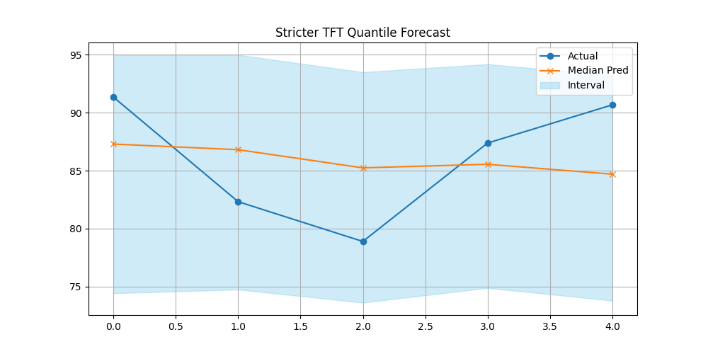
Visualization of the quantile forecast using the stricter TFT model.

Discussion of Exercise

In this exercise, you explored quantile forecasting with two TFT variants:

1. Flexible `TemporalFusionTransformer`: Demonstrated with only dynamic inputs, showcasing its adaptability. Inputs are provided as [None, dynamic_array, None].

2. Stricter `TFT`: Showcased with all three input types (static, dynamic, future) generated via make_multi_feature_time_series() and prepared using reshape_xtft_data(). Inputs are provided as [static_array, dynamic_array, future_array].

Key takeaways include:

• Setting the quantiles parameter in the model’s __init__ method.

• Using combined_quantile_loss() for training.

• Understanding that the model’s output shape changes to include the number of quantiles.

• Visualizing prediction intervals to assess forecast uncertainty.

This exercise provides a foundation for building more complex probabilistic forecasting models.