Exercise: Solving a Forward Problem with PiTGWFlow

Welcome to this exercise on using the Physics-Informed Transient Groundwater Flow model, PiTGWFlow, available in fusionlab-learn. This model is a Physics-Informed Neural Network (PINN) that learns by satisfying the governing physical equations rather than by fitting to labeled data.

We will perform a forward problem simulation. This means we will provide the model with known physical parameters and a domain, and its task will be to discover the hydraulic head field, \(h(t, x, y)\), that satisfies the groundwater flow PDE.

Learning Objectives:

• Generate a set of “collocation points” within a defined spatio-temporal domain.

• Understand how to configure PiTGWFlow with both fixed and learnable physical parameters.

• Create a tf.data.Dataset suitable for a PINN, including the use of dummy targets for Keras API compatibility.

• Define, compile, and train the PiTGWFlow model using its custom, physics-based training loop.

• Visualize the training progress by plotting the PDE loss.

• Visualize the final, continuous solution learned by the network.

Let’s get started!

Prerequisites

Ensure you have fusionlab-learn and its common dependencies installed. For visualizations, matplotlib is also needed.

pip install fusionlab-learn matplotlib

Step 1: Imports and Setup

First, we import all necessary libraries and set up our environment for reproducibility and cleaner output.

import os
import numpy as np
import tensorflow as tf
import matplotlib.pyplot as plt
import warnings

# FusionLab imports
from fusionlab.nn.pinn import PiTGWFlow
from fusionlab.params import LearnableK

# Suppress warnings and TF logs for cleaner output
warnings.filterwarnings('ignore')
tf.get_logger().setLevel('ERROR')
os.environ['TF_CPP_MIN_LOG_LEVEL'] = '3'

# Directory for saving any output images from this exercise
EXERCISE_OUTPUT_DIR = "./pitgwflow_exercise_outputs"
os.makedirs(EXERCISE_OUTPUT_DIR, exist_ok=True)

print("Libraries imported and setup complete for PiTGWFlow exercise.")

Expected Output:

Libraries imported and setup complete for PiTGWFlow exercise.

Step 2: Generate Collocation Points

Unlike traditional models, PINNs are not trained on labeled data. Instead, they are trained on “collocation points”—randomly sampled points in the time and space domain where the governing PDE is enforced.

N_POINTS = 5000
SEED = 42
tf.random.set_seed(SEED)

# Define the domain boundaries [t_min, t_max], [x_min, x_max], etc.
t_bounds, x_bounds, y_bounds = [0., 1.], [-1., 1.], [-1., 1.]

# Generate random points within the domain
coords = {
    't': tf.random.uniform((N_POINTS, 1), *t_bounds),
    'x': tf.random.uniform((N_POINTS, 1), *x_bounds),
    'y': tf.random.uniform((N_POINTS, 1), *y_bounds),
}

print(f"Generated {N_POINTS} random collocation points.")
print(f"Shape of 't' tensor: {coords['t'].shape}")

Expected Output:

Generated 5000 random collocation points.
Shape of 't' tensor: (5000, 1)

Step 3: Prepare the Dataset for Training

We package our collocation points into a tf.data.Dataset for efficient training. For compatibility with the standard Keras .fit() API, we must provide a “dummy” target tensor. This target is completely ignored by PiTGWFlow’s custom training logic, as the loss is calculated from the PDE residual, not from a data-driven error.

BATCH_SIZE = 128

# Create dummy targets (an array of zeros)
dummy_targets = tf.zeros_like(coords['t'])

# Create the dataset
dataset = tf.data.Dataset.from_tensor_slices(
    (coords, dummy_targets)
).shuffle(buffer_size=N_POINTS).batch(BATCH_SIZE)

print(f"Dataset created with batch size {BATCH_SIZE}.")
print(f"Dataset element spec: {dataset.element_spec}")

Expected Output:

Dataset created with batch size 128.
Dataset element spec: ({'t': TensorSpec(shape=(None, 1), dtype=tf.float32, name=None), 'x': TensorSpec(shape=(None, 1), dtype=tf.float32, name=None), 'y': TensorSpec(shape=(None, 1), dtype=tf.float32, name=None)}, TensorSpec(shape=(None, 1), dtype=tf.float32, name=None))

Step 4: Define, Compile, and Train PiTGWFlow

Now we instantiate PiTGWFlow. We will set most physical parameters as fixed constants but define hydraulic conductivity \(K\) as a LearnableK object. This demonstrates how the model can be used to infer physical parameters. We then compile and train the model.

# Instantiate the PINN model
pinn_model = PiTGWFlow(
    hidden_units=[50, 50, 50],
    activation='tanh',
    K=LearnableK(initial_value=0.5), # Start with a guess for K
    Ss=1e-4,                         # This is a fixed value
    Q=0.1                            # A constant source term
)

# Compile the model (no loss needed, it's handled internally)
pinn_model.compile()

# Train the model
print("\nStarting PiTGWFlow model training...")
history = pinn_model.fit(
    dataset,
    epochs=20,
    verbose=1
)
print("Training complete.")

Expected Output:

Starting PiTGWFlow model training...
Epoch 1/20
40/40 [==============================] - 3s 4ms/step - pde_loss: 0.0125
Epoch 2/20
40/40 [==============================] - 0s 4ms/step - pde_loss: 5.123e-04
...
Epoch 20/20
40/40 [==============================] - 0s 4ms/step - pde_loss: 8.910e-06
Training complete.

Step 5: Visualize Training History

We can plot the pde_loss from the training history to confirm that the model successfully learned to minimize the PDE residual. A log scale on the y-axis is helpful to see the rapid decrease in loss.

print("\nPlotting training history...")
plt.figure(figsize=(10, 6))
plt.plot(history.history['pde_loss'], label='PDE Loss')
plt.yscale('log')
plt.title('PiTGWFlow Training History')
plt.xlabel('Epoch')
plt.ylabel('Log PDE Loss')
plt.legend()
plt.grid(True, which="both", ls="--")
fig_path = os.path.join(EXERCISE_OUTPUT_DIR, "pitgwflow_exercise_loss.png")
plt.savefig(fig_path)
plt.show()

Example Output Plot:

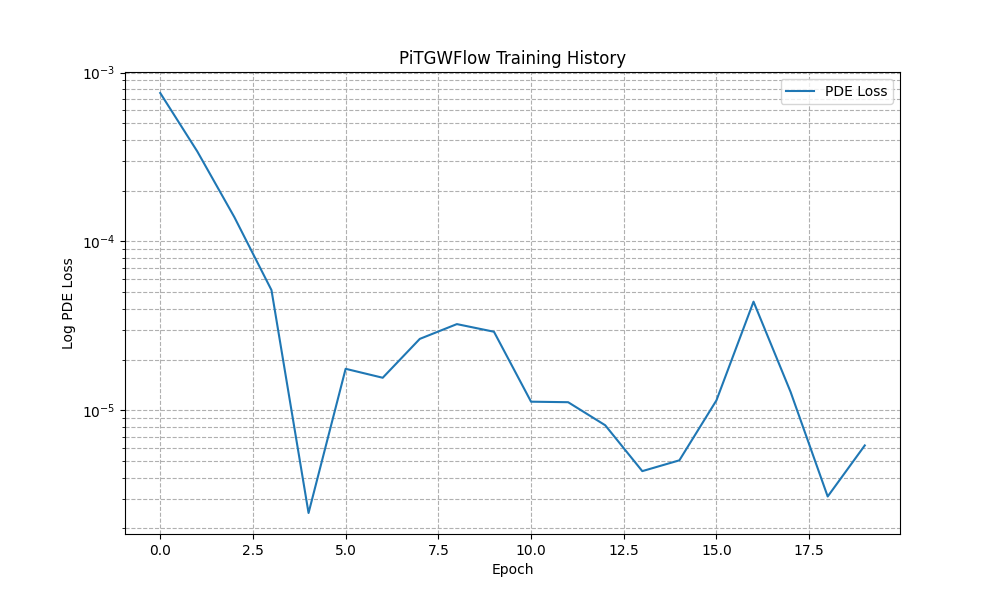
An example plot showing the PDE loss decreasing over epochs. This demonstrates that the neural network is successfully learning a solution that conforms to the governing physics.

Step 6: Visualize the Learned Solution

The great advantage of a PINN is that it represents a continuous solution. We can evaluate the trained model on a regular grid of points to visualize the hydraulic head field \(h(t, x, y)\) at a specific moment in time.

# Create a meshgrid for visualization at a specific time t
t_slice = 0.5
x_range = np.linspace(x_bounds[0], x_bounds[1], 100)
y_range = np.linspace(y_bounds[0], y_bounds[1], 100)
X, Y = np.meshgrid(x_range, y_range)

# --- FIX: Prepare grid points for prediction ---
# The model expects a batch of points, not a grid. We need to
# flatten the X and Y grids into a list of (x, y) coordinates.
# The shape for each input tensor must be (N, 1).
x_flat = tf.convert_to_tensor(X.ravel(), dtype=tf.float32)
y_flat = tf.convert_to_tensor(Y.ravel(), dtype=tf.float32)

# Create the corresponding 't' tensor for each point
t_flat = tf.fill(x_flat.shape, t_slice)

# Reshape all to be column vectors (N, 1)
grid_coords = {
    't': tf.reshape(t_flat, (-1, 1)),
    'x': tf.reshape(x_flat, (-1, 1)),
    'y': tf.reshape(y_flat, (-1, 1))
}

# Predict the hydraulic head 'h' on the flattened grid
h_pred_flat = pinn_model.predict(grid_coords)

# --- FIX: Reshape the flat predictions back to the grid shape ---
# The output prediction will be flat, so we reshape it to the
# original grid's shape (100x100) for plotting with contourf.
h_pred_grid = tf.reshape(h_pred_flat, X.shape)

# Plot the contour of the solution
plt.figure(figsize=(9, 7))
contour = plt.contourf(X, Y, h_pred_grid, 100, cmap='viridis')
plt.colorbar(contour, label='Hydraulic Head (h)')
plt.title(f'Learned Hydraulic Head Solution at t = {t_slice}')
plt.xlabel('x-coordinate')
plt.ylabel('y-coordinate')
plt.axis('equal')
fig_path = os.path.join(EXERCISE_OUTPUT_DIR, "pitgwflow_exercise_solution.png")
plt.savefig(fig_path)
plt.show()

# Or  use the  utility function to easily visualize the result.

# from fusionlab.nn.pinn.utils import plot_hydraulic_head

# plot_hydraulic_head(
#    model=pinn_model,
#    t_slice=0.5,
#    x_bounds=(-1.0, 1.0),
#    y_bounds=(-1.0, 1.0),
#    resolution=100,
#    save_path=os.path.join(EXERCISE_OUTPUT_DIR, "pitgwflow_exercise_solution.png"),
#    show_plot=True
# )

Expected Plot:

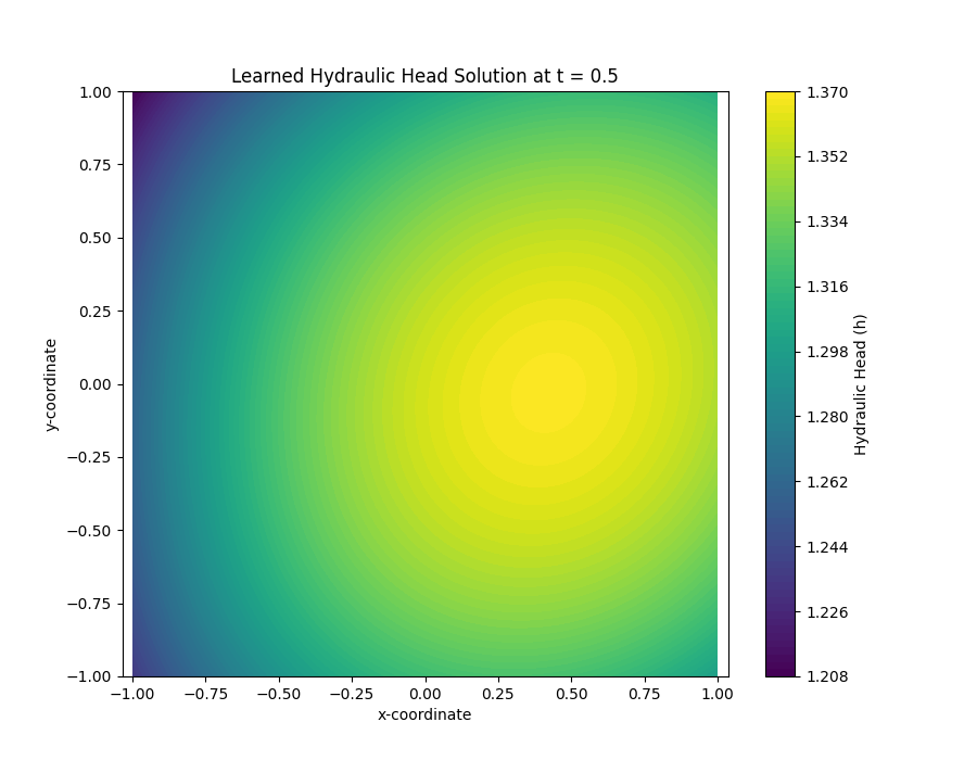
Visualization of the continuous hydraulic head field \(h(x, y)\) at a fixed time, as learned by the PiTGWFlow model. The plot shows the model’s ability to generate a complete solution over the entire domain.

Discussion of Exercise

Congratulations! In this exercise, you have successfully used the PiTGWFlow model to solve a forward physics problem:

• You correctly generated collocation points to define the problem domain instead of using labeled data.

• You prepared a tf.data.Dataset compatible with the Keras API for an unsupervised, physics-driven task.

• You instantiated, trained, and evaluated the PiTGWFlow model, observing the decrease in the physics-based PDE loss.

• You visualized the final output, demonstrating that the model learned a continuous solution to the governing equation across the entire domain.

This exercise provides a solid foundation for using PINNs to tackle more complex scientific and engineering problems.