Quickstart (end-to-end)

This walkthrough runs a minimal end-to-end experiment in GeoPrior v3.2: load a dataset, prepare tensors (Stage-1), train a baseline model (Stage-2), run inference, and inspect results.

If you have not installed the GUI yet, start with Installation and startup.

Before you begin

• Make sure you can launch the app (see Installation and startup).

• Decide a results root folder. GeoPrior will store every run (Stage-1, Train, Tune, Inference, Transfer) under that root. The full layout is documented in Output folders and file layout.

• Have at least one dataset available (either already in your library for Auto scan or as a CSV ready to import).

Tip

Keep Dry run enabled the first time you click through the workflow. It lets you verify your configuration and paths in the log panel without executing Stage-1/Stage-2.

Main window at a glance

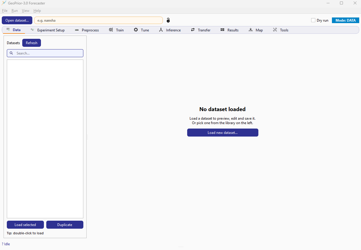
GeoPrior v3 main window. The tab strip drives the workflow and the log panel records every action and configuration used.

Step 1 — Select a dataset (Data tab)

1. Go to the Data tab.

2. Choose your data source:

   • Auto scan: select a dataset from the library list on the left. Double-click a dataset (or use Load selected).

   • Manual import: use Open dataset… (top-left) to import a CSV into your dataset library.

3. Confirm that the dataset preview area updates and that the log panel reports the selected dataset key/path.

Note

The dataset you select becomes the default input for later tabs. If you switch datasets mid-workflow, you usually want to re-run Stage-1 (Preprocess) to keep manifests and tensors consistent.

Step 2 — Define the experiment (Experiment Setup tab)

1. Open Experiment Setup.

2. Set the core time configuration:

   • Training end year (end of observed history)

   • Forecast start year

   • Forecast horizon (how many future years to predict)

   • Time steps (sequence length used by the model)

3. Review/adjust training basics:

   • epochs, batch size, learning rate

   • device mode (auto/cpu/gpu) if exposed by your build

4. Make sure the city name matches the dataset you intend to run (the city field in the top bar is a convenient shortcut).

Tip

If you are unsure, keep defaults and only change: training end year, forecast start year, and horizon. That is enough for a minimal reproducible run.

Step 3 — Run Stage-1 preprocessing (Preprocess tab)

Stage-1 prepares everything Stage-2 needs:

• normalized tensors / NPZ files

• scalers

• a Stage-1 manifest (paths + metadata)

1. Open Preprocess.

2. Choose/confirm the output location under your results root.

3. Run Stage-1.

4. Watch the log panel until you see a clear “completed” message and a path to the created Stage-1 folder/manifest.

What to verify:

• A Stage-1 run directory exists under the results root.

• A manifest file is written (used later by Train/Inference).

• Optional future NPZ is produced if “build future” is enabled.

Warning

If you change training years, horizon, feature columns, or normalization settings after Stage-1, re-run Stage-1. Otherwise Stage-2 may train/infer on mismatched tensors.

Step 4 — Train a baseline model (Train tab)

1. Open Train.

2. Confirm that Stage-1 artifacts are detected (or browse to a manifest if your UI provides a manual selector).

3. Start a baseline training run (Stage-2).

4. Monitor progress in the log panel. Use the global Stop button if you need to interrupt a long run.

What you get:

• a trained model file (e.g., .keras)

• training logs and metrics

• optional evaluation artifacts if enabled in your build

Tip

For your first run, keep epochs modest (e.g., 5–20) to validate the pipeline end-to-end, then increase once everything is stable.

Step 5 — (Optional) Tune hyperparameters (Tune tab)

Use Tune when you want a better model than the baseline.

1. Open Tune.

2. Review the tuning overview (search space summary).

3. Adjust trials/epochs (and any tuner settings exposed).

4. Run tuning and wait for the best trial to be reported.

5. Save/record the best configuration and model output path.

Note

Tuning can be expensive. For quick validation, start with a small number of trials and short epochs.

Step 6 — Run inference and export forecasts (Inference tab)

Inference generates predictions using a trained model.

1. Open Inference.

2. Select the model file (baseline or tuned).

3. Choose the inference input:

   • Validation/Test/Train split (uses Stage-1 tensors), or

   • Custom NPZ if you are providing external inputs.

4. For forecasting mode, enable Use Stage-1 future NPZ (if your Stage-1 created it).

5. Configure export options (CSV/NPZ/plots) as available.

6. Run inference and confirm output paths in the log panel.

What to verify:

• a forecast CSV is written (for inspection/sharing)

• optional NPZ outputs exist (for downstream analysis)

• plots are generated if enabled

Step 7 — Inspect outputs and metrics (Results tab)

1. Open Results.

2. Refresh/scan the results root.

3. Use filtering/search to locate the city/run you just created.

4. Open tables/plots and verify key metrics and files.

5. (Optional) Download a run as a ZIP for sharing or archiving.

Tip

If you work across multiple results roots, use the Results tab’s view-root switching (when available) to browse without changing the configured results root.

Step 8 — (Optional) Cross-city transferability (Transfer tab)

Transferability evaluates how well a model trained on City A performs on City B, with optional calibration and rescaling.

1. Open Transfer.

2. Set City A (source) and City B (target).

3. Choose splits (val/test) and calibration modes (none/source/target).

4. Run the transfer matrix job and confirm that CSV/JSON outputs are produced under the results root.

5. Use the built-in view generation (if enabled) to create a summary figure/panel.

Step 9 — (Optional) Spatial inspection (Map tab)

Use Map to explore spatial patterns in subsidence and uncertainty.

1. Open Map.

2. Select a run/output layer (prediction, residuals, uncertainty).

3. Use the analytics panels (e.g., sharpness/reliability/inspector) to validate calibration and spatial consistency.

4. Export figures if your UI provides export controls.

Step 10 — Tools (Tools tab)

The Tools tab groups utilities that help you inspect, validate, and reuse the artifacts produced by Stage-1/Stage-2, without rerunning the full workflow. It is especially useful when you have many cities and runs under the same results root and want to quickly pick the “right” manifest/model, check configuration drift, or generate reproducible batch scripts.

Tools tab. The left list contains tool modules (Stage-1 manager, device monitor, inspectors, generators). The main panel shows the currently selected tool (here: Stage-1 manager).

Tool library (left panel)

The left panel is a searchable tool library. Each entry opens a dedicated tool in the main workspace.

Typical tools include:

• Stage-1 manager: browse Stage-1 runs/manifests by city, inspect what was produced, and select a preferred manifest for subsequent Train/Tune/Inference steps.

• GPU / device monitor: confirm which compute device will be used before launching Stage-2 jobs.

• Config inspector & diff: compare the current GUI configuration against a saved JSON config/manifest and highlight differences.

• Manifest browser & validator: inspect train/tune/inference manifests and validate integrity (missing files, mismatched metadata).

• Dataset explorer: quick dataset health checks (shape, coverage, missing values).

• Paths & permissions: verify data/results roots and write access.

• Script / batch generator: generate reproducible CLI scripts from the current configuration for batch runs.

• Metrics dashboard: visualize diagnostics such as reliability/PIT and other metrics when outputs are available.

Stage-1 manager (main workspace)

When Stage-1 manager is selected, the main workspace is split into two parts:

1. Available Stage-1 runs (table)

2. Selected manifest summary (key/value panel)

Workflow:

1. Click Refresh to scan the configured results roots for Stage-1 runs and manifests.

2. Use Filter by city to narrow the table (for example, when you have many cities).

3. Click a row to select a Stage-1 run. The lower panel updates with a compact config summary and the most relevant artifact paths.

4. Click Use for this city in GUI to set the selected Stage-1 run as the preferred input for downstream tabs (Train/Tune/Inference).

This is the fastest way to “pin” the correct Stage-1 artifacts when you have multiple runs with similar settings.

Quick actions and command palette

The Tools tab also exposes lightweight shortcuts:

• A Quick toolbar (icons) for common actions.

• A command palette (Type a command...) that lets you search and run tool actions by name (for example, typing a keyword such as metrics).

Use these when you want to jump directly to a tool or action without scrolling through the tool list.

When to use Tools

Use the Tools tab when you need to:

• audit which Stage-1 run produced a given set of tensors/manifests,

• detect configuration drift between runs,

• validate manifests before long training/tuning jobs,

• confirm device selection before Stage-2,

• export or regenerate scripts for reproducibility.

In short: Workflow tabs run jobs; Tools help you manage and verify the artifacts those jobs create.

Use these tools when you want to automate runs, share a configuration, or standardize experiment reproduction.

Reproducibility note

Note

Every action is logged to the log panel, and the configuration used for each run is saved alongside the outputs. This makes experiments reproducible and auditable. See Configuration key reference and Output folders and file layout.