Experiment Setup tab
The Experiment Setup tab is the configuration center of GeoPrior v3. It collects all run-critical settings (paths, time window, data semantics, model/training knobs, physics constraints, probabilistic outputs, tuning, device/runtime) into a single, store-backed workspace.
Unlike the Data tab (which focuses on dataset selection and preview), Experiment Setup focuses on declaring intent: what experiment you want to run, with what semantics, and with which defaults or overrides.
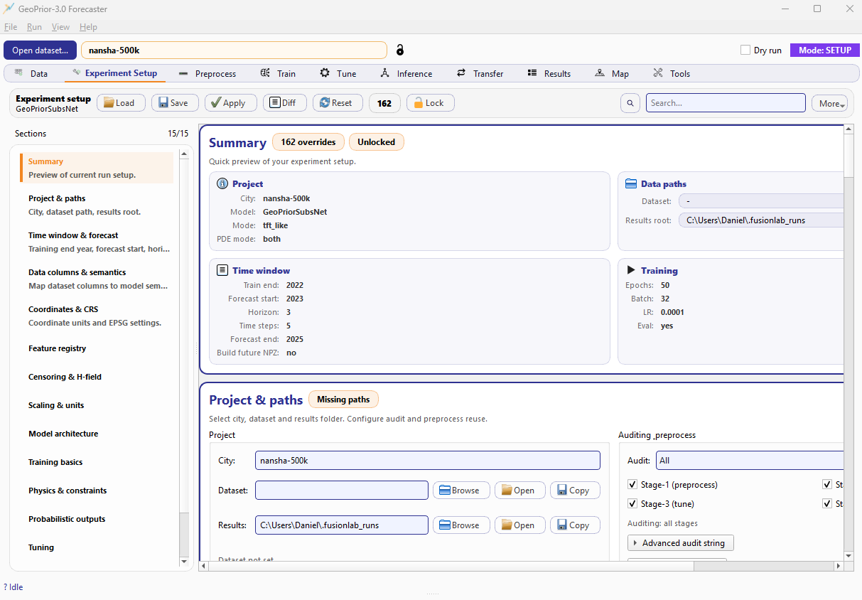
Experiment Setup tab. A sticky header (actions + search + lock), a left navigation with sections, and a right scroll area with section cards (Summary, Paths, Time window, Data semantics, etc.).
What this tab controls
The Experiment Setup tab is the single place where you define:
Project context: city name, model name, dataset path, results root.
Time window & forecast: training end year, forecast start, horizon, time steps, and whether to build a future NPZ.
Data columns & semantics: mapping dataset columns to model roles (time, lon, lat, subsidence, GWL, H-field, head proxy settings, etc.).
Coordinates & CRS: coordinate mode (degrees/meters), EPSG settings, normalization rules.
Architecture / training / physics / probabilistic outputs: the knobs that define the Stage-2 model run.
Tuning and runtime: hyperparameter tuning settings and device/ runtime preferences.
The key idea is that these choices are saved as a reproducible config snapshot and are reused by downstream tabs (Preprocess, Train, Tune, Inference, Transfer, Results, Map).
Layout overview
The tab is composed of three parts:
1) Sticky header (actions + search + lock)
At the top you will see a compact header with:
Load: import a configuration snapshot (JSON) and patch it into the current configuration.
Save: save the current config snapshot to the last used JSON path.
Apply: broadcast the current config to the rest of the GUI so other tabs refresh immediately (useful after bulk edits).
Diff: view the current override diff (what changed relative to the baseline/default config).
Reset: restore defaults (use with care).
Overrides counter: the pill showing how many keys differ from the baseline (example:
162 overrides).Lock: toggle read-only mode for the entire setup panel.
Search + More: filter sections/cards by text and access extra actions (export/copy helpers, depending on build).
This header is designed to make configuration management explicit: you can quickly see whether the setup is “clean”, how many overrides are active, and whether editing is currently locked.
Note
Load/Save here refer to configuration snapshots (JSON). They do not load datasets. Datasets are loaded in the Data tab.
3) Right scroll area (cards)
The main workspace is a scrollable stack of cards, one per section. Cards are presented in the same order as the navigation list.
Each card typically contains:
a title (matching the section),
an optional status pill (e.g., Missing paths, Unlocked),
grouped widgets with labels and tooltips,
and immediate feedback (validation state, detected dataset columns, etc., depending on the card).
Config store and overrides
GeoPrior v3 uses a single configuration store as the source of truth. Every widget change patches one or more keys in that store.
Two concepts are visible in the UI:
Snapshot: the full configuration as a JSON-friendly dict.
Overrides (diff): only the keys that differ from the baseline defaults.
That’s why you see an “overrides count” pill in the header. It is a lightweight audit indicator: a run with many overrides is not “bad”, but it reminds you the configuration is far from defaults and should be saved as a snapshot for reproducibility.
Tip
Use Diff before long training or tuning runs. It is the fastest way to verify you did not accidentally change something critical (years, horizon, semantics, physics weights, etc.).
Locking the setup (prevent accidental edits)
The Lock button turns the setup panel into a read-only view. This is useful when you are:
inspecting an existing run setup,
browsing multiple sections without wanting to change values,
presenting a configuration (screenshots/demos),
or using the tab as an “audit dashboard”.
When locked, widgets are disabled and the header shows the lock state (e.g., Unlocked vs locked). Unlock when you are ready to edit again.
Recommended workflow
A minimal but reliable workflow is:
In Data, select or import your dataset.
In Experiment Setup, verify the three essentials:
Project & paths: city, dataset path, results root.
Time window & forecast: train end, forecast start, horizon, time steps (and future NPZ toggle).
Data columns & semantics: confirm the correct time/lon/lat/target columns and GWL semantics.
Click Apply to refresh dependent tabs immediately.
Continue to Preprocess (Stage-1), then Train/Tune/Inference.
If you change any of the essentials after running Stage-1, re-run Stage-1 to keep artifacts consistent.
Warning
Changing time window, horizon, or column semantics after Stage-1 can invalidate previously generated tensors/manifests. If you are unsure, rerun Stage-1 in the Preprocess tab.
Key cards you will use most
Summary
The Summary card provides a compact, read-only preview of your current experiment setup: city, model, mode, PDE mode, dataset path, results root, and the most important time/training settings. It is meant to answer, at a glance: “What run am I about to launch?”
Project & paths
The Project & paths card defines the identity of the experiment and the workspace where artifacts will be written. It is intentionally the first “real” section after Summary, because every other stage (Stage-1/Train/Tune/Infer/Transfer) depends on these paths being stable.
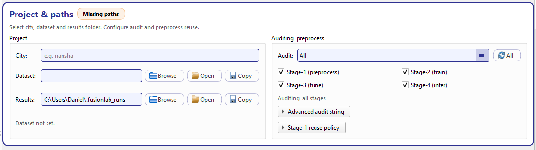
Project & paths. Left: city + dataset/results path pickers. Right: audit stage presets and Stage-1 reuse policy.
Project (left group)
The left side contains three fields:
- City
A free text identifier used to label runs and to organize outputs under your results root. This value is stored as
cityand is used across the GUI (tab header, manifests, folder naming, reporting). The field accepts any string, but keeping it consistent with your dataset naming (e.g.,nansha-500k) makes browsing runs much easier.- Dataset
A read-only path field bound to
dataset_path. Use Browse to pick a CSV file. Once set, two convenience actions are available:Open: open the dataset path in the operating system file browser.
Copy: copy the dataset path to the clipboard (useful for bug reports or external scripts).
The dataset path is part of the run “contract”: if it is not set, the card shows a warning badge and the hint text will report Dataset not set.
- Results
A path field bound to
results_root. This is the root directory under which GeoPrior stores all stage outputs and exported artifacts. It behaves like the dataset row:Browse selects the results folder.
Open opens it in the OS.
Copy copies it to the clipboard.
This field is editable, but the recommended workflow is to pick it with Browse to avoid typos.
At the bottom of this group, the card continuously validates the two critical paths and renders an explicit hint:
If dataset is missing: Dataset not set.
If results root is missing: Results root not set.
If both exist: Paths look good.
The section header shows a badge such as Missing paths until both paths are present, then switches to Ready.
Auditing & preprocess (right group)
The right side of the card controls two related ideas:
Audit selection (what stages should produce audit metadata)
Stage-1 reuse policy (how to treat existing Stage-1 artifacts)
Audit presets + checkboxes
The Audit drop-down provides quick presets:
Off: disable auditing
Preprocess: audit Stage-1 only
Train + tune: audit Stage-2 and Stage-3
All: audit every stage
Custom: preserve your manual selection
Below the preset selector, you have explicit checkboxes for each stage:
Stage-1 (preprocess)
Stage-2 (train)
Stage-3 (tune)
Stage-4 (infer)
This dual design is intentional: presets are fast, but the checkboxes are transparent. Whenever you click checkboxes, the preset will automatically switch to Custom if the selection does not match a known preset.
Under the hood, the selection is encoded into a single store key
audit_stages:
*means “all stages”otherwise a comma-separated list like
stage1,stage2,stage3
This encoding is visible and editable in Advanced audit string, which is an expander that exposes a raw text box for power users.
A small hint line summarizes the current mode, e.g. Auditing: all stages or Auditing: stage1,stage3. :contentReference[oaicite:1]{index=1}
Stage-1 reuse policy (expander)
The Stage-1 reuse policy expander mirrors the same controls used in the Preprocess tab, but places them here so you can decide reuse/rebuild behavior at configuration time (before you run Stage-1).
Clean Stage-1 dir (
clean_stage1_dir): clears the Stage-1 run directory before rebuilding. Use this when you suspect stale files or want a clean, reproducible rebuild.Auto reuse if match (
stage1_auto_reuse_if_match): reuse an existing compatible Stage-1 run when configuration matches. This saves time and avoids regenerating tensors unnecessarily.Force rebuild if mismatch (
stage1_force_rebuild_if_mismatch): if a Stage-1 run exists but does not match the current configuration, rebuild automatically instead of continuing with potentially inconsistent artifacts.
These options matter because Stage-1 is the “data contract” for Stage-2: a mismatch between the current setup and the Stage-1 manifest is one of the most common causes of confusing downstream behavior.
Time window & forecast
The Time window & forecast card defines the temporal scope of the experiment and provides immediate feedback to prevent inconsistent windows (for example, forecasting that starts before training ends).
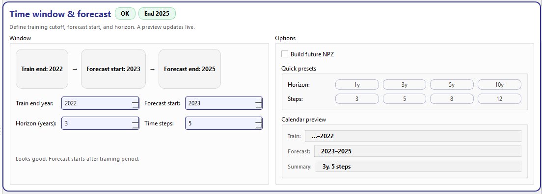
Time window & forecast. Left: timeline preview and core year fields. Right: options, quick presets, and a calendar preview.
Window (left group)
The left side is designed for “read it like a timeline”:
- Timeline preview
A compact visual chain:
Train end → Forecast start → Forecast endThese values update live as you change the spin boxes.
- Core fields
Train end year (
train_end_year): the final observed year included in the training history.Forecast start (
forecast_start_year): the first predicted year (must be greater than Train end year).Horizon (years) (
forecast_horizon_years): how many years to forecast into the future.Time steps (
time_steps): the lookback length / sequence size used to build model inputs for Stage-2.
The card computes Forecast end as:
forecast_end = forecast_start_year + forecast_horizon_years - 1
and displays it both in the timeline and as a badge (e.g. End 2025).
- Validation hint
The card validates that
forecast_start_year > train_end_yearand displays a friendly hint:If valid: Looks good. Forecast starts after training period.
If invalid: Forecast start should be greater than train end year.
The top badge switches between OK and Check accordingly.
Options (right group)
Build future NPZ
Build future NPZ (build_future_npz) controls whether Stage-1
creates the “future-known” NPZ payload used by forecasting mode.
Enable this when you plan to run forward forecasts beyond the training
range and want inference to consume a standardized “future” tensor set.
Quick presets
The Quick presets block provides one-click buttons for common configurations:
Horizon presets: 1y, 3y, 5y, 10y
Time steps presets: 3, 5, 8, 12
These buttons simply patch the corresponding store keys, but they make it much easier to standardize runs across cities (especially when comparing transferability).
Calendar preview
The Calendar preview block turns the numeric settings into an interpretation-friendly summary:
Train: shows the end of the training range (e.g.,
…–2022)Forecast: shows the forecast window (e.g.,
2023–2025)Summary: compact meta (e.g.,
3y, 5 steps)
These labels are selectable (copy/paste) and update live as you change any of the core fields. :contentReference[oaicite:5]{index=5}
Data columns & semantics
The Data columns & semantics card is where you bind your dataset to GeoPrior’s required roles and explicitly declare the meaning conventions used by key variables (especially subsidence and groundwater level). This is the bridge between “a CSV with columns” and “a model-ready dataset”.
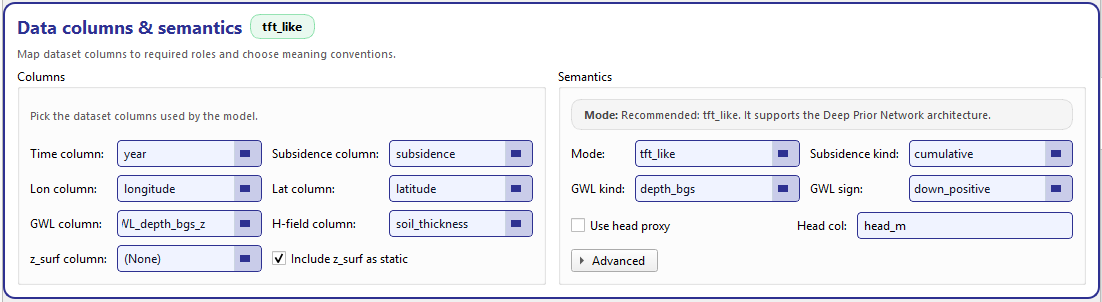
Data columns & semantics. Left: dataset column pickers. Right: semantic conventions (mode, kinds, sign) + head proxy options.
Columns (left group)
The left side contains role-to-column pickers. Each field is a combo box that is populated from the active dataset columns (provided by the Data tab), but remains editable, so you can type a column name manually when needed.
The core roles are:
- Time column
The temporal index used to assemble sequences (typically
year).- Lon / Lat columns
The spatial coordinates of each sample (used both for modeling and for map inspection later).
- Subsidence column
The target variable for forecasting (e.g.,
subsidence).- GWL column
Groundwater-level measurement used as a dynamic driver. The semantics (depth vs head, sign convention) are configured on the right side.
- H-field column
Optional hydro/geo field used by the physics or feature registry (for example, soil thickness). If not used, you can leave it unset.
- z_surf column
Optional surface elevation used when deriving head proxies or when you want elevation as a static feature. The field supports a “none” option, and the checkbox below controls whether it is included in the static feature stack.
- Include z_surf as static
When checked, GeoPrior will treat
z_surfas a static variable even if it is stored as a regular column in the dataset. This is useful when elevation is constant per location and you want it available to the model without being repeated as a dynamic sequence.
Note
These pickers do not rename your CSV by themselves. They define the mapping used by Stage-1/Stage-2. If you want to permanently normalize column names, do it in the Data tab (Save / Save as) so future runs stay consistent.
Semantics (right group)
The right side defines meaning conventions. This is critical because many geoscience datasets encode the same physical quantity in different ways (depth vs head, positive up vs positive down, cumulative vs incremental).
Subsidence kind
Subsidence kind declares how your target column is encoded:
cumulative: the value represents accumulated subsidence up to that year
(other options may exist depending on your schema)
This matters for how Stage-1 builds training targets and how Results/Map interpret temporal plots.
GWL kind + GWL sign
These two controls define the groundwater convention:
- GWL kind
Declares what the GWL column represents (for example, depth below ground surface vs hydraulic head). In your screenshot the UI shows
depth_bgs(depth below ground surface).- GWL sign
Declares the sign convention. In your screenshot,
down_positivemeans larger values correspond to deeper water level (more depth).
These settings must match your dataset; otherwise you can end up with physically inverted behavior (e.g., drawdown interpreted as rise).
Use head proxy + head column
Some workflows prefer to work with head directly (meters) instead of depth below surface. The Use head proxy checkbox enables a head-derivation path, and Head col lets you specify the column name to use when head is already available (or when you want Stage-1/Stage-2 to reference a derived head field). The head column entry is a plain text field (with a placeholder) and is bound to the configuration store so it is saved with your run artifacts.
Advanced (expander)
The Advanced expander contains optional settings that are not needed for a basic run. One important example is GWL dynamic index: it is implemented as an optional integer (a “Set” checkbox + a spin box). You only enable it when you need explicit indexing behavior for the GWL channel in a dynamic stack.
Coordinates & CRS
The Coordinates & CRS card controls how GeoPrior interprets spatial coordinates and (when needed) how it converts them into a modelling-friendly CRS (typically a planar UTM grid). This card is split into CRS settings (left) and an always-on preview + helpers panel (right).
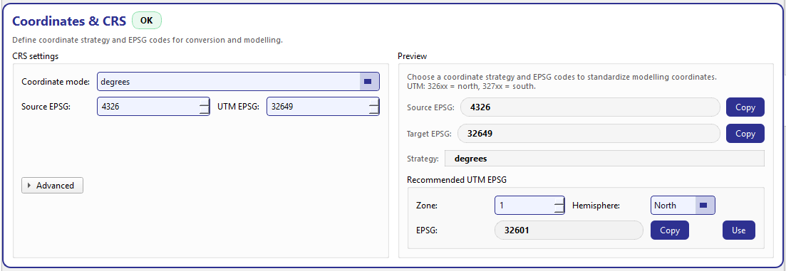
Coordinates & CRS. Left: coordinate mode and EPSG settings with advanced toggles. Right: effective CRS preview, copy buttons, and a UTM recommender.
CRS settings (left group)
Coordinate mode
Coordinate mode selects the overall strategy (for example, keep lon/lat in degrees, or project/convert to a planar CRS such as UTM). The combo is store-driven and not editable, so your choice is always one of the supported strategies. :contentReference[oaicite:7]{index=7}
Source EPSG + UTM EPSG
The card uses an EPSG pair:
- Source EPSG
The CRS your dataset coordinates are currently in (commonly
4326for WGS84 lon/lat). If your dataset is already well-defined and standard, set it here so conversions are explicit and auditable.- UTM EPSG
The target planar CRS used when the selected coordinate mode requires UTM. The UI calls it “UTM EPSG”, but functionally it is your target EPSG for modelling coordinates.
Advanced (expander)
The Advanced expander contains compact toggles that influence how coordinates are stored and normalized:
normalize_coords: apply coordinate normalization (useful for stable model training when values are large).
keep_coords_raw: keep the original coordinates available in addition to modelling coordinates.
shift_raw_coords: apply a shift to raw coordinates (useful when you want a local origin).
These flags are intentionally “advanced”: most users can keep defaults unless they have a strong reason (e.g., comparing multiple cities with different coordinate scales).
Preview + UTM helper (right group)
Effective CRS preview
The preview panel continuously displays:
Source EPSG and Target EPSG (with Copy buttons),
Strategy (a human-readable description of the chosen mode),
a status badge (OK or Check) with a short hint message.
For example, if you choose a UTM conversion strategy but leave the target EPSG unset, the badge switches to Check and the hint explains that UTM conversion requires a target UTM EPSG.
Recommended UTM EPSG
The card includes a built-in UTM recommender:
Choose a Zone (1–60) and Hemisphere (North/South).
The UI computes the EPSG using the standard rule:
32600 + zonefor North32700 + zonefor South
It then shows the recommended EPSG with Copy and Use actions:
Copy puts the recommended EPSG on the clipboard.
Use fills the target/UTM EPSG field in the left panel with this value.
A subtle hint is also shown in the preview: UTM: 326xx = north, 327xx = south. This makes it harder to accidentally pick the wrong hemisphere.
Tip
If your dataset is in lon/lat degrees (EPSG:4326) and you plan to run spatially-aware physics or map diagnostics, using a planar CRS (UTM) often makes distances and gradients behave more naturally. Use the recommender to avoid memorizing EPSG codes.
Feature registry
The Feature registry card provides a modern, typo-safe way to select feature columns from the active dataset and register them into the configuration store. The key design choice is simple: users select only from dataset columns (no free typing), so feature lists remain consistent across runs and do not break because of spelling mistakes.
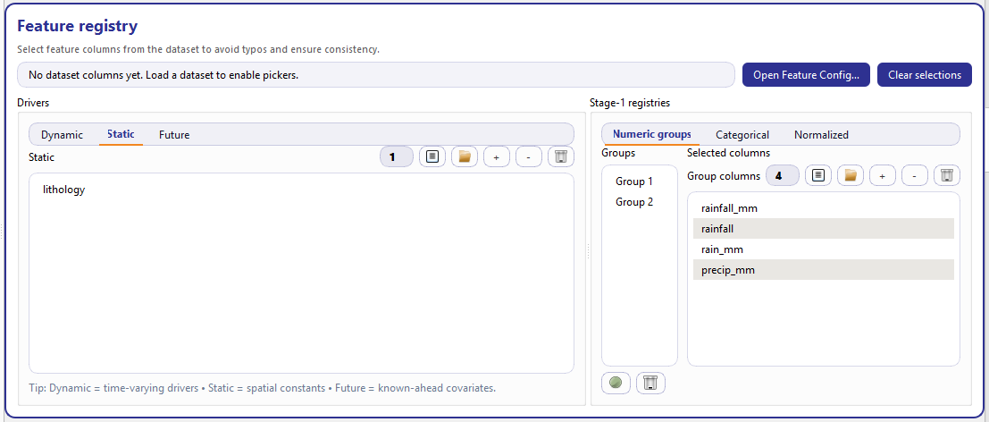
Feature registry. Left: model drivers (Dynamic/Static/Future). Right: Stage-1 registries (Numeric groups / Categorical / Normalized).
What the registry controls
This card writes directly into store-backed lists that are used by Stage-1 and Stage-2:
dynamic_driver_features: time-varying covariates (per time step)static_driver_features: spatial constants (per location)future_driver_features: known-ahead covariates (available for the forecast horizon)optional_numeric_features: numeric groups (list-of-lists)optional_categorical_features: categorical feature registryalready_normalized_features: features that should be treated as already normalized and excluded from some scaling steps
All changes are committed via store.patch(...), so selections are
persisted in the same configuration snapshot used everywhere in the GUI.
Top bar: status + shortcuts
At the top of the card you see:
- Status message
A live message indicating whether dataset columns are available and whether all selected features are valid.
If no dataset is loaded: No dataset columns yet. Load a dataset to enable pickers.
If everything is valid: Dataset columns: N. All selected features are valid.
If there are issues: Some selected features are not in the dataset: … and the tooltip lists all missing names.
This status is computed by checking all selected feature lists against the available dataset columns. :contentReference[oaicite:2]{index=2}
- Open Feature Config…
Opens the dedicated FeatureConfigDialog (advanced configuration). This dialog is important because it can edit not only the registries, but also several related keys (drivers, censor flags, time/lon/lat columns, etc.) in one place. For now, think of the registry card as the “fast picker” UI, and the dialog as the “power editor”.
- Clear selections
Clears all registries in one click by patching empty lists to each store key. This is useful when switching datasets or when you want to restart feature selection from scratch. :contentReference[oaicite:4]{index=4}
Drivers (left panel)
The left side (“Drivers”) defines the covariates that the model will consume, grouped by how they behave over time.
It is implemented as a tabbed selector with three lists:
Dynamic features are time-varying drivers (e.g., rainfall, pumping, groundwater depth) that can change each year/time step. They become part of the dynamic input tensor produced in Stage-1 and consumed by Stage-2.
Static features are spatial constants that do not change over the time axis (e.g., geology class, lithology, building concentration if treated as static). They typically appear once per location and are broadcast over time inside the model.
Future features are known-ahead covariates available for the forecast horizon (e.g., planned controls, scenario variables, calendar features). They allow the model to condition forecasts on inputs that are known in advance.
A short hint line below the tabs summarizes this meaning directly in the UI: Dynamic = time-varying drivers • Static = spatial constants • Future = known-ahead covariates. :contentReference[oaicite:5]{index=5}
Stage-1 registries (right panel)
The right side (“Stage-1 registries”) is also tabbed, and focuses on how Stage-1 should interpret subsets of features during preprocessing.
Numeric groups is a list-of-lists editor used to declare groups of
numeric columns. Conceptually, this lets you register sets of features
that should be handled together (for example, a “rainfall family” of
columns such as rainfall_mm, rainfall, precip_mm).
The UI has two parts:
a left list of groups (Group 1, Group 2, …)
a “Group columns” editor for the currently selected group
You can add/remove groups and reorder columns within a group (drag and
drop). All changes are committed to optional_numeric_features as a
nested list structure.
Categorical is a registry of optional categorical columns. It is a
simple multi-selection list bound to optional_categorical_features.
This registry is used by Stage-1 to treat these columns as categorical
signals (rather than scaling them as numeric).
Normalized registers columns that are already normalized (for example,
features that are known to be in a stable [0, 1] range or that were
pre-scaled externally). These are stored in
already_normalized_features and allow Stage-1 to avoid applying
redundant scaling transformations.
The typo-safe multi-select editor
Every list in this card uses the same safe editor component:
it receives the available dataset columns via
set_available(cols)it stores the current selection in a reorderable list
it offers a compact set of actions in the header
Each list shows a title, a count badge, and action buttons:
Pick (replace): opens a searchable dialog and replaces the whole selection with the new choice.
Paste: reads the clipboard and adds only valid column names (accepts comma/space/newline separated input; case-insensitive mapping to canonical dataset column names).
+ Add: opens the picker and appends selected columns.
− Remove: removes selected items.
Trash: clears the list.
All list changes update the count badge immediately, and (when dataset
columns exist) the UI can show a small “missing chip” (!N) if any
selected columns are not present in the dataset. Hovering the chip shows
which names are missing.
Why this matters (and common usage patterns)
When you load a dataset, the card becomes “enabled” because it now has the canonical list of columns. This eliminates the most common source of silent bugs: feature name typos.
When you switch datasets, the status line and missing chips help you immediately see which selected features do not exist in the new file.
The Paste action is a productivity feature: it lets you copy a column list from a paper/notes/CSV header and only keeps the columns that truly exist.
Numeric groups provide a clean way to keep “families” of related covariates together for auditing and Stage-1 handling.
Note
The Feature registry is a selection layer. It does not modify the CSV itself. To permanently rename or edit columns, use the Data tab (Save / Save as). The registry only records which columns should be treated as drivers/registries for a given experiment snapshot.
Feature configuration dialog
The Feature configuration dialog is the “power editor” behind the Feature registry. It is designed to configure, in one place, the columns and feature lists that GeoPriorSubNet (PINN) needs for Stage-1 and Stage-2.
Compared to the registry card (which focuses on safe selection from lists), this dialog emphasizes fast mapping, auto-matching, and censoring (H-field) controls.
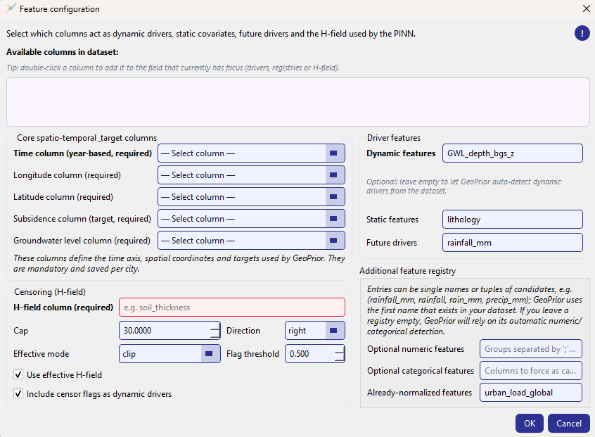
Feature configuration dialog. Top: available columns (double-click to insert). Left: required core columns + H-field censoring. Right: driver features and optional registries.
Available columns (top box)
The top panel lists all dataset columns in a read-only view. A key workflow feature is double-click insertion: double-clicking a column name inserts it into the field that currently has focus (drivers, registries, or H-field).
This is implemented by tracking the last focused field (via an event filter) and then applying a mode-specific insertion rule:
CSV fields (dynamic/static/future/normalized/categorical): append as comma-separated values (duplicates are ignored).
Optional numeric registry: add as a new group separated by
;.H-field: replaces the entire value (single required column).
Core spatio-temporal & target columns (required)
This group defines the minimal contract between your dataset and GeoPrior. All fields are required and are selected from non-editable combo boxes:
Time column (year-based, required)
Longitude column (required)
Latitude column (required)
Subsidence column (target, required)
Groundwater level column (required)
Auto-mapping behavior
When the dialog opens, it attempts to map default names from configuration
(e.g., year, longitude, latitude, subsidence,
GWL_depth_bgs_z) to the dataset columns using a robust name-matching rule:
Case-insensitive match on a normalized form (underscores/punctuation ignored)
Fuzzy match using
difflib.get_close_matches(cutoff ≈ 0.75)
If no “year” mapping is found, the dialog may preselect a time-like column containing tokens such as “date”, “month”, “week”, or “time”, and displays a one-time information message reminding that the current workflow expects an annual (year-based) time axis. :contentReference[oaicite:4]{index=4}
Validation styling
Required fields are validated live. Missing required fields are highlighted with a red border and tinted background. On OK, the dialog blocks closing and shows a “Required features missing” message listing what must be set (core columns and the H-field).
Driver features
This group defines the primary feature lists consumed by the model:
- Dynamic features
Time-varying drivers used by the temporal encoder (e.g., GWL depth, rainfall, pumping). The UI text notes that this field can be left empty to allow GeoPrior to auto-detect dynamic drivers from the dataset, but the dialog’s help and validation rules emphasize that the model needs a sensible dynamic input set for meaningful runs. :contentReference[oaicite:6]{index=6}
- Static features
Spatial constants that do not vary over time (e.g., lithology, geology class).
- Future drivers
Known-ahead covariates used during forecasting (e.g., rainfall forecasts).
All three fields are comma-separated lists, and the double-click insertion mechanism makes it easy to build these lists from the available columns panel.
Additional feature registry
The registry fields provide fine-grained hints to Stage-1 about how to treat columns, especially when column names differ across cities/datasets.
A distinctive capability here is candidate tuples: each registry entry can be either a single name or a group of candidate names. The registry parser uses:
;to separate groups,to separate candidates within a group
Example input:
rainfall_mm, rainfall, rain_mm, precip_mm; urban_load_global, urban_load
This becomes two groups:
(rainfall_mm, rainfall, rain_mm, precip_mm) and
(urban_load_global, urban_load).
GeoPrior then uses the first name that exists in the dataset. If none of the candidates exist, the group is dropped (registry filtered to dataset-safe names). :contentReference[oaicite:9]{index=9}
The dialog exposes three registry fields:
- Optional numeric features
Groups of numeric candidates (often used to stabilize naming across datasets).
- Optional categorical features
Columns (or candidate groups) you want to force as categorical.
- Already-normalized features
Columns that should be treated as already scaled and therefore skipped (or treated specially) by scaling logic. :contentReference[oaicite:10]{index=10}
If registries are left empty and a full DataFrame is available, the dialog can infer reasonable defaults from dtypes and cardinality (numeric vs categorical) as a fallback.
Censoring
This section configures the H-field used by the PINN physics and how censored values are handled.
- H-field column (required)
Column name for the physical field (e.g., soil thickness). This field is required; missing H-field blocks closing the dialog on OK.
- Cap
Censoring threshold (default around
30.0). Values beyond the cap may be treated as censored depending on direction and mode.- Direction
Whether censoring applies on the
righttail (large values) orlefttail (small values).- Effective mode
How the effective H-field is produced for censored samples:
clip: clamp to the capcap_minus_eps: clamp slightly below the capnan_if_censored: set censored entries to NaN (downstream logic must handle missingness)
- Flag threshold
Threshold used for setting censor flags (default around
0.5).
Two checkboxes control how the model uses this information:
Use effective H-field: use the transformed effective H-field.
Include censor flags as dynamic drivers: append censor indicators to the dynamic driver channels.
See more details in Censoring & H-field.
What this dialog saves (overrides)
When you click OK, the dialog produces a dictionary of configuration overrides (used by the GUI/store) that includes:
core column keys:
TIME_COL,LON_COL,LAT_COL,SUBSIDENCE_COL,GWL_COLdriver lists:
DYNAMIC_DRIVER_FEATURES,STATIC_DRIVER_FEATURES,FUTURE_DRIVER_FEATUREScensoring keys:
H_FIELD_COL_NAME,CENSORING_SPECS, andUSE_EFFECTIVE_H_FIELD/INCLUDE_CENSOR_FLAGS_AS_DYNAMICregistries (only if non-empty):
OPTIONAL_NUMERIC_FEATURES_REGISTRY,OPTIONAL_CATEGORICAL_FEATURES_REGISTRY,ALREADY_NORMALIZED_FEATURES
Because these values are saved into the same store-backed configuration as the rest of the GUI, the exact feature choices (and censoring policy) are preserved next to run artifacts for reproducibility and auditing.
Censoring & H-field
The Censoring & H-field card defines censor rules for the H-field (typically a thickness/height field used by the PINN), and optionally generates derived columns:
a flag column that marks censored samples, and
an effective H-field column that replaces/adjusts censored values.
This card is store-driven and persists its full configuration under:
censoring_specs(list of rule dicts),use_effective_h_field(bool),include_censor_flags_as_dynamic(bool),include_censor_flags_as_future(bool).
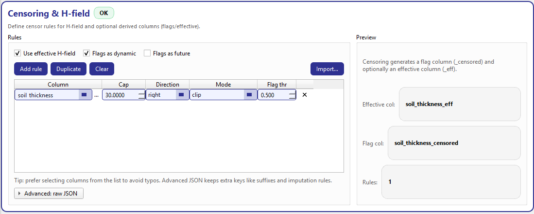
Censoring & H-field. Left: rule editor (table + advanced JSON). Right: live preview of derived column names and rule count.
Why censoring exists in GeoPrior v3
H-field values (e.g., soil_thickness) often contain outliers, hard caps
from measurement protocols, or physically implausible tails. Censoring
lets you encode a clear policy for how these values are handled, while
keeping the policy auditable (saved into the run configuration and
manifest context).
Rules (left panel)
The left panel is the primary workflow. It avoids raw JSON typing as the default path and provides a structured rule table driven by dataset columns.
At the top of the Rules panel, three compact toggles control how derived outputs are produced and consumed by the model:
- Use effective H-field
When enabled, Stage-1/Stage-2 can use an
*_effversion of the H-field (based on the rule’seff_mode). When disabled, the effective column is not produced/used, even if rules exist.- Flags as dynamic
When enabled, a censor flag channel (
*_censoredby default) can be included in the dynamic driver stack. This is useful if censoring events have temporal structure and you want the model to “see” them.- Flags as future
When enabled, the censor flag can be included in the future-known driver stack when applicable. :contentReference[oaicite:3]{index=3}
The toolbar provides the standard rule editing workflow:
Add rule: append a new rule initialized from a template (or from the first rule if one already exists).
Duplicate: copy the selected rule and insert it right after.
Clear: remove all rules.
Import…: import censoring specs from the Feature configuration dialog (when available), so you can configure censoring once and reuse it.
Each row defines one censoring rule and is stored as a dict inside
censoring_specs. The table columns map to these fields:
- Column
The dataset column to censor (your H-field). This cell is a combo box populated from dataset columns. It is also editable so power users can paste a name, but it is validated against the known dataset columns.
A small “…” button opens a searchable column picker to avoid typos.
- Cap
The censoring threshold (float). Values beyond the cap (depending on Direction) are treated as censored.
- Direction
Which tail is censored: -
rightfor high values (e.g., thickness > cap), -leftfor low values (e.g., thickness < cap).- Mode
How the effective column is produced for censored samples: -
clip: clamp to the cap, -cap_minus_eps: clamp slightly below cap (useful to avoid equalityeffects in later logic),
nan_if_censored: set censored entries to NaN (downstream processing must handle missingness).
- Flag thr
Threshold used to compute a censor flag (float in [0, 1]). Default is 0.5.
- ✕
Remove the rule. :contentReference[oaicite:5]{index=5}
The card validates that each rule’s Column exists in the current dataset column list. If a row is invalid, the Column combo is styled with a red border and shows a tooltip: Pick a valid dataset column. This prevents silent errors when switching datasets or renaming columns. :contentReference[oaicite:6]{index=6}
Advanced: raw JSON (optional)
The Advanced: raw JSON expander exposes the full-fidelity JSON list that backs the table. This is intentionally optional: the table is the recommended workflow, but JSON is available when you need to preserve or add extra keys.
Two actions are provided:
Copy: copy the JSON payload to clipboard.
Apply JSON: parse JSON and overwrite
censoring_specs(expects a list of dicts). :contentReference[oaicite:7]{index=7}
Note
The table editor focuses on the “common” keys (col/cap/direction/eff_mode/
flag_threshold). JSON allows additional keys to be preserved such as:
flag_suffix, eff_suffix, and any future extension fields (for example,
imputation hints). The card is designed to keep these extra keys intact.
Preview (right panel)
The Preview panel gives immediate feedback about what Stage-1 will generate.
- Derived column names
The preview shows:
Effective col: derived as
<col><eff_suffix>ifuse_effective_h_fieldis enabled. Default suffix is_eff.Flag col: derived as
<col><flag_suffix>. Default suffix is_censored.
The suffixes are read from the first rule when present (keys
eff_suffixandflag_suffix); if not provided, defaults are used.- Rules count
Displays how many rules exist in
censoring_specs.- Status badge
The badge summarizes validity:
Missing: no rules are defined (with a hint encouraging you to add one).
Check: rules exist but some rows have invalid columns.
OK: rules exist and at least the primary column looks valid.
Import workflow (from Feature configuration)
The Import… button opens the Feature configuration dialog and, if that dialog provides censoring overrides, imports them directly into:
censoring_specs(fromCENSORING_SPECS), and optionallyinclude_censor_flags_as_future(if exposed by the dialog).
This keeps the two UIs consistent: you can configure censoring once in the dialog and then review/edit the same rules in this dedicated card.
Practical example
A common configuration is a single rule on soil_thickness with:
cap = 30.0
direction = right
mode = clip
flag threshold = 0.5
This produces:
soil_thickness_eff(if effective H-field is enabled)soil_thickness_censored(always, once a rule exists)
and you can optionally append the flag channel into dynamic/future drivers depending on the checkboxes.
Scaling & units
The Scaling & units card is one of the most important pieces of the GeoPrior v3 setup because it controls how raw dataset values are interpreted, normalized, and converted into physically consistent (SI-compatible) quantities for the PINN.
In practice, this card bridges two worlds:
Stage-1 scaling (data preprocessing) decides which fields are scaled/normalized when Stage-1 builds tensors and scalers.
SI affine mapping (physics + model consistency) defines how your dataset units are converted into SI-like values using simple affine formulas (multiply + scale + bias), so physics residuals and learned closures behave consistently across datasets and cities.
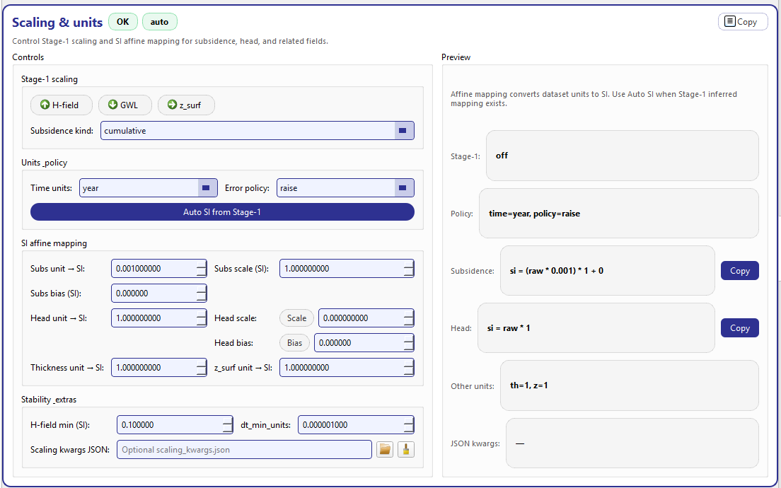
Scaling & units: left side edits scaling and SI mapping; right side previews the resulting formulas and status.
What this card controls
This card edits store-backed keys such as:
Stage-1 toggles:
scale_h_field,scale_gwl,scale_z_surfTemporal units + safety:
time_units,scaling_error_policyAuto/manual SI mapping:
auto_si_affine_from_stage1SI affine parameters:
subs_unit_to_si,subs_scale_si,subs_bias_si,head_unit_to_si, optionalhead_scale_si, optionalhead_bias_si, plusthickness_unit_to_si,z_surf_unit_to_siStability extras:
h_field_min_si,dt_min_unitsAdvanced override:
scaling_kwargs_json_path(optional JSON).
Stage-1 scaling (chips)
At the top of the card you see three checkable “chips” (pill toggles):
H-field
GWL
z_surf
These toggles control whether Stage-1 applies scaling/normalization logic to each field when generating Stage-1 artifacts (normalized arrays, scalers, and manifest metadata). Turning a chip on/off updates the store immediately and is reflected in the Preview column under Stage-1.
Subsidence kind
Subsidence kind selects how subsidence values should be interpreted:
cumulative: the dataset column is cumulative subsidence (monotonic accumulation over time, in the dataset’s native unit).rate: the dataset column is a per-time-step rate.
This choice matters because it changes how Stage-1 and Stage-2 interpret time differencing and consistency checks.
Units & policy
This block defines two global safety controls:
- Time units
Declares the unit of the time axis for scaling logic (supported:
year,day,second). It is used to interpretdtand time-based scaling consistently. :contentReference[oaicite:4]{index=4}- Error policy
Controls what happens when scaling settings look inconsistent:
raise(recommended): stop and force you to fix the issuewarn: continue but log a warningignore: continue silently (use carefully)
The preview will warn you when policy is permissive (e.g., ignore).
Auto SI from Stage-1
The Auto SI from Stage-1 toggle (checkable button) is the recommended default when you have a valid Stage-1 run for the current city/dataset.
When enabled, Stage-2 can reuse SI/scale hints inferred and saved during Stage-1 (via manifest metadata), instead of relying purely on manual entries. This reduces drift across runs and is especially useful when sharing Stage-1 artifacts across team members or machines.
Note
Auto SI does not “guess physics.” It simply prefers Stage-1’s saved mapping when it exists, making re-runs and reloading more consistent.
SI affine mapping (the core concept)
The SI affine mapping section defines how raw dataset values are converted before being used by physics-aware parts of the model.
The general pattern is shown explicitly in the Preview:
- Subsidence
si = (raw * subs_unit_to_si) * subs_scale_si + subs_bias_si
A common example is subsidence stored in millimeters (mm). In that case,
subs_unit_to_si = 0.001 converts mm → meters, while scale and bias
often remain 1 and 0. :contentReference[oaicite:7]{index=7}
- Head
Head uses the same idea, but with optional scale and bias:
si = raw * head_unit_to_si [* head_scale_si] [+ head_bias_si]
In the UI, Scale and Bias are explicit toggles: if you do not enable them, the corresponding value is treated as “not applied” and is not included in the formula. This avoids accidental double-scaling.
- Other units
Two additional unit-to-SI multipliers are provided:
Thickness unit → SI (often used for H-field units)
z_surf unit → SI (elevation / surface height, if used)
The Preview summarizes them compactly (e.g., th=1, z=1).
Stability & extras
This compact section contains small but important stability controls:
- H-field min (SI)
A lower bound used to avoid numerically problematic near-zero thickness in physics computations.
- dt_min_units
A minimum time step in the chosen time units. This acts as a guard against division-by-small-dt effects when differencing or computing residual terms. :contentReference[oaicite:10]{index=10}
Scaling kwargs JSON (advanced override)
Scaling kwargs JSON lets you point to an optional JSON file that overrides (or enriches) computed scaling settings.
The underlying pipeline supports precedence-based overrides and performs safety checks (for example, it can reject a JSON override that was built for a different dynamic feature layout when strict checks are enabled).
Use this feature when you need to:
lock a known-good scaling configuration for a production run,
reproduce a published experiment exactly,
share scaling settings across machines without copying full manifests.
Preview (right column)
The Preview column is intentionally “copy-friendly” and reflects exactly what your current settings imply:
Stage-1: which Stage-1 scalings are active (or
off)Policy:
time=<...>, policy=<...>Subsidence formula (with a Copy button)
Head formula (with a Copy button)
Other units summary
JSON kwargs path (or
—)
Two small badges also help you diagnose state quickly:
status:
OKvsCheckdepending on basic validityauto:
auto(Stage-1 mapping preferred) vsmanual.
Recommended workflow
Load your dataset and ensure the time/targets/semantics are correct.
Run Stage-1 once (Preprocess tab) to produce a manifest.
Enable Auto SI from Stage-1 to reuse inferred mapping.
Only switch to manual SI parameters if you are certain the Stage-1 mapping is incomplete or you need a controlled override.
Keep
scaling_error_policy=raiseuntil you are confident the setup is stable; relax towarnonly when needed.
Model architecture
The Model architecture card controls the main neural backbone and the core dimensional knobs used by GeoPriorSubNet. It is intentionally split into two layers:
On-card “core” controls for the most common parameters (fast to tune).
A full Architecture configuration dialog (opened via Configure… or Architecture config…) for advanced attention settings and detailed overrides (documented later in Architecture configuration dialog).
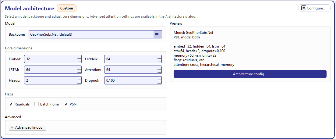
Model architecture: left side edits the backbone and core dimensions; right side previews the effective configuration and opens the full Architecture configuration dialog.
Backbone (model selector)
The Backbone selector lists the available model families and their roadmap status. In v3.2 you will see:
GeoPriorSubsNet(default, current)PoroElasticSubsNet(next)HybridAttn(future)
When a roadmap item is selected (PoroElasticSubsNet or HybridAttn),
the GUI does not silently switch models. Instead, it shows a banner
message explaining that the backbone is not yet available and applies a
controlled fallback:
For
PoroElasticSubsNetthe app keepsGeoPriorSubsNetand setspde_mode='consolidation'to approximate consolidation-only physics.For
HybridAttnthe app keepsGeoPriorSubsNetand setspde_mode='off'(disabling physics) to mimic a pure attention run.
If you return to the default backbone explicitly, the card restores the previous PDE mode you had before the fallback was applied. This behavior prevents accidental configuration drift while still letting you explore the roadmap options safely.
Core dimensions
The Core dimensions box exposes the parameters most users adjust during experimentation. These are bound directly to the configuration store and update the preview live. The default ranges are intentionally bounded to avoid unstable configurations.
- Embed
embed_dim— embedding width used to project inputs into the model feature space (range: 8–512).- Hidden
hidden_units— hidden width used in main blocks (range: 8–1024).- LSTM
lstm_units— recurrent width used by temporal components when enabled (range: 8–1024).- Attention
attention_units— attention projection width (range: 8–512).- Heads
num_heads— number of attention heads (range: 1–16).- Dropout
dropout_rate— dropout probability (0.0–0.90, step 0.01).
Flags
The Flags box enables/disables common architectural features:
- Residuals
use_residuals— adds residual connections for stability.- Batch norm
use_batch_norm— enables batch normalization in supported blocks.- VSN
use_vsn— enables a Variable Selection Network (feature gating).
When VSN is disabled, the related VSN size knob in Advanced is also disabled (greyed out) to make dependencies explicit.
Advanced knobs (expander)
The Advanced knobs expander holds less frequently used parameters:
- Memory
memory_size— size of memory state used by attention/memory mechanisms (range: 1–512).- VSN units
vsn_units— internal width of the VSN (range: 4–512), only enabled when VSN is checked.
Preview (effective configuration)
The right-side Preview box is the “source of truth” summary and updates live whenever the store changes. It includes:
selected model name,
PDE mode (important when fallbacks apply),
a compact line summary of embed/hidden/lstm/attention/heads/dropout,
memory + vsn_units,
enabled flags (residuals / batch-norm / vsn),
attention levels (e.g., cross / hierarchical / memory).
In addition, the card shows a badge (top-right of the card header) that indicates whether your architecture is Default or Custom. The badge turns to Custom when any of the architecture-related store keys are overridden (embed_dim, hidden_units, dropout_rate, attention_levels, etc.).
Architecture config button (reference)
There are two ways to open the same advanced dialog:
the card header action Configure…
the preview button Architecture config…
Both open the full ArchitectureConfigDialog, which exposes detailed attention-level configuration and additional advanced options.
We document that dialog next, including the meaning of “attention levels” and how overrides are mapped into store keys:
See Architecture configuration dialog.
Architecture configuration dialog
The Architecture configuration dialog is the advanced editor opened from the Model architecture card (via Configure… or Architecture config…). It exposes the attention layout and the core architectural knobs used by the GeoPriorSubNet “BaseAttentive” backbone, while keeping the UI compact and safe.
A key design detail is that the dialog returns only the keys you actually changed (a minimal “delta”), so your configuration remains clean and the Default / Custom status is meaningful.
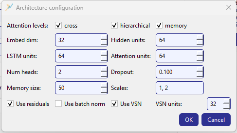
Architecture configuration dialog for GeoPriorSubNet.
What this dialog edits
This dialog edits a focused subset of the NATCOM-style configuration:
ATTENTION_LEVELSEMBED_DIM,HIDDEN_UNITS,LSTM_UNITS,ATTENTION_UNITSNUMBER_HEADS,DROPOUT_RATEMEMORY_SIZE,SCALESUSE_RESIDUALS,USE_BATCH_NORM,USE_VSN,VSN_UNITS
When you click OK, these keys are mapped back into the GUI/store keys:
ATTENTION_LEVELS→attention_levelsEMBED_DIM→embed_dimHIDDEN_UNITS→hidden_unitsLSTM_UNITS→lstm_unitsATTENTION_UNITS→attention_unitsNUMBER_HEADS→num_headsDROPOUT_RATE→dropout_rateMEMORY_SIZE→memory_sizeSCALES→scalesUSE_*/VSN_UNITS→ corresponding boolean/units keys.
Attention levels (the most important switch)
The top row lets you enable one or more attention levels:
cross
hierarchical
memory
At least one level must be selected; the dialog blocks closing and shows a warning if all three are unchecked. :contentReference[oaicite:3]{index=3}
- cross
Cross-feature/context attention. Use this when you want the model to integrate information across drivers and representations at the same temporal scale (a strong default).
- hierarchical
Multi-scale attention behavior. Pair this with meaningful Scales (see below) if your system benefits from coarse-to-fine temporal context.
- memory
Enables memory-style attention and uses Memory size as a controlling capacity knob. This is useful when long-range dependencies matter or when you want the model to retain a compact history summary beyond the LSTM window.
For most GeoPrior runs, a safe and expressive default is enabling
cross + hierarchical + memory with moderate dimensions (as shown
in the screenshot). If you need a lighter model:
Start by disabling memory (and reduce Memory size),
then reduce Hidden units / Attention units,
only then reduce Embed dim.
Core dimensions
The dialog exposes the same primary dimensions as the on-card controls, but in one place:
Embed dim (8–512): projection width into the model space.
Hidden units (8–1024): main hidden capacity.
LSTM units (8–1024): recurrent capacity (sequence modeling).
Attention units (8–512): attention projection capacity.
Num heads (1–16): number of attention heads.
Dropout (0.0–0.9): regularization strength.
Increasing Hidden / Attention generally increases capacity and compute cost.
Increasing Heads improves representation diversity but can destabilize training if combined with very small attention units.
Use Dropout conservatively (0.05–0.20 is typical); large dropout can slow convergence.
Memory & scales
These two knobs work together with the attention levels:
- Memory size
(1–512) controls the capacity when memory attention is enabled.
- Scales
A comma-separated integer list (e.g.
1, 2). This is parsed into a list of ints and saved asSCALES. If parsing fails, the dialog blocks closing and shows a “Scales must be integers” message.
Think of Scales as the model’s multi-resolution schedule. A common
starting point is 1, 2 (two levels). For deeper hierarchical context you
might use 1, 2, 4 (but be aware this increases compute and the risk of
overfitting).
Flags: residuals, batch norm, VSN
Three checkboxes toggle common architecture features:
- Use residuals
Residual connections improve stability and are recommended in most cases.
- Use batch norm
Batch normalization may help for some datasets but can interact with sequence modeling; enable it only if you have evidence it improves training.
- Use VSN
Enables Variable Selection Network (feature gating). If enabled, you can tune VSN units (4–512).
Saving behavior (clean overrides)
When you press OK, the dialog:
Builds the current configuration dict from widget values.
Compares it against the initial values used to open the dialog.
Returns only changed keys via
get_overrides().
That delta is then mapped into store keys and patched, which is why:
the preview in the Model architecture card updates immediately, and
the “Custom” badge reflects real overrides rather than repeating defaults.
Recommended setup workflow
Start from defaults:
cross + hierarchical + memory, moderate dims.Adjust capacity in this order: Hidden units → Attention units → Heads → Embed.
If training is unstable, increase Dropout slightly (e.g. +0.02–0.05), and keep Use residuals on.
Keep Scales small (
1, 2) until you have evidence multi-scale modeling improves results.Enable VSN when you have many drivers and want the model to learn feature relevance; keep VSN units near your embed size as a first guess.
Training basics
The Training basics card centralizes the core optimization loop settings used by Train and Tune, plus the runtime switches that affect what gets exported and how TensorFlow executes on your machine.
This card is fully store-driven: every widget is bound to
GeoConfigStore, and
the current values are also surfaced as compact “badges” in the card
header (epochs, batch size, learning rate, and optional flags such as
SavedModel / In-mem / Debug).
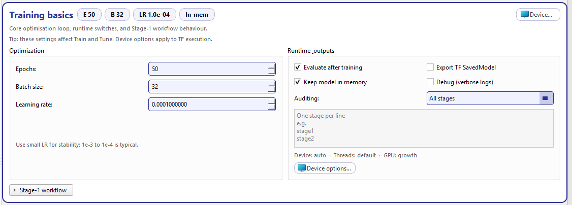
Training basics: optimization parameters on the left, runtime & outputs on the right, with auditing controls and device/runtime options.
Optimization (core loop)
This panel defines the training loop parameters:
- Epochs
Total number of epochs used during training/tuning. The control supports a wide range (1 → 100000) and steps by 5 for quick iteration.
- Batch size
Mini-batch size (1 → 8192). The step size is 8 to make it easy to move through typical powers-of-two choices.
- Learning rate
The optimizer learning rate (
1e-10→10.0) with 10 decimals. The card also displays a stability note: 1e-3 to 1e-4 is typical for stable runs. :contentReference[oaicite:1]{index=1}
Runtime & outputs
These toggles control what happens after training and what artifacts are kept/exported:
- Evaluate after training
If enabled, the training run triggers evaluation at the end (so metrics and summaries are produced automatically).
- Keep model in memory
Keeps the in-memory model object available for immediate follow-up actions in the same session (useful for quick inference or inspection without reloading).
- Export TF SavedModel
Exports a TensorFlow SavedModel in addition to the native
.kerasmodel (useful for deployment or external tooling that expects SavedModel).- Debug (verbose logs)
Enables extra logging. It is surfaced as a header badge (
Debug) so you can immediately see when verbose mode is active.
Auditing
Auditing controls how run steps are recorded/validated across pipeline stages. The UI supports three modes:
- All stages
Sets
audit_stages="*"(audit everything).- Off
Sets
audit_stages=""(no auditing).- Custom list
Enables a small text editor where you write one stage name per line, e.g.:
stage1
stage2
The card stores this as a list of strings. When the store value is a list, the UI auto-switches into “Custom list” and repopulates the editor.
Device preview (live summary)
Below auditing, the card shows a compact runtime summary computed from device-related store keys, e.g.:
Device: auto · Threads: default · GPU: growth
This preview is updated whenever device keys change (device mode, thread counts, GPU memory policy). :contentReference[oaicite:4]{index=4}
Stage-1 workflow (expander)
The Stage-1 workflow expander mirrors the Stage-1 behavior flags used during preprocessing reuse and forecasting preparation:
Clean Stage-1 directory before run (
clean_stage1_dir)Auto reuse if config matches (
stage1_auto_reuse_if_match)Force rebuild if mismatch (
stage1_force_rebuild_if_mismatch)Pre-build future_* NPZ (Stage-3) (
build_future_npz)
These are the same “guard rails” you see in the Preprocess workflow: they control whether Stage-1 artifacts can be reused safely between runs and whether future-known tensors are prepared ahead of time. x=5}
Device & runtime dialog
The Device & runtime dialog (opened via Device options… in the card or via the header action Device…) configures TensorFlow execution: device selection, CPU threading, and GPU memory behavior.
A crucial UX detail: this dialog uses rollback on Cancel. When the dialog opens, it snapshots device keys; if you press Cancel, all changes made while the dialog was open are reverted automatically.
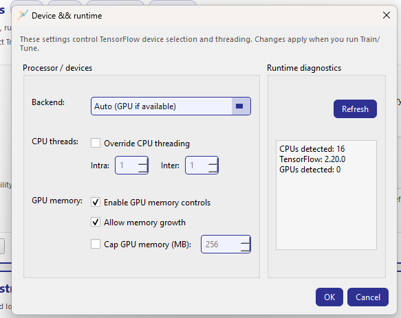
Device & runtime: hardware selection and execution policies for TensorFlow, plus live diagnostics.
Processor / devices
- Backend
Select the execution backend:
Auto (GPU if available): choose GPU when available, otherwise CPU.
Other modes (when supported by your build) typically include CPU-only or explicit GPU selection.
- CPU threads
Optional override for TensorFlow thread pools:
Override CPU threading enables manual control.
Intra: threads within an operation.
Inter: threads across independent operations.
If you do not override, the preview in Training basics shows
Threads: default.
- GPU memory
Controls TensorFlow GPU allocation strategy:
Enable GPU memory controls activates the section.
Allow memory growth tells TF to allocate GPU memory progressively.
Cap GPU memory (MB) sets a hard memory limit (when enabled).
These settings correspond to store keys such as
tf_gpu_allow_growth and tf_gpu_memory_limit_mb and are reflected
in the Training basics device preview as GPU: growth and/or
cap=<N>MB.
Runtime diagnostics
The right panel provides a quick environment check (with Refresh):
CPU count detected
TensorFlow version
GPU count detected
This is meant as a sanity check when users report “GPU not used” or when thread overrides are applied. :contentReference[oaicite:9]{index=9}
When changes take effect
Device/runtime settings apply when you launch Train or Tune. They do not retroactively change an already-running job. The reason is that TensorFlow device placement and threading are typically configured at session/runtime initialization, so GeoPrior applies these settings at job start for consistency. :contentReference[oaicite:10]{index=10}
Physics & constraints
The Physics & constraints card is the control center for GeoPrior’s physics-informed training. It lets you decide when PDE residuals are used, how they are computed, what bounds to enforce on learned physical fields, and how strongly each loss component contributes to optimization.
The card is intentionally “at a glance”: the most common switches and weights are inline, while deeper edits are delegated to two dedicated dialogs:
Edit physics… →
PhysicsConfigDialogScalars & losses… →
ScalarsLossDialog:contentReference[oaicite:0]{index=0}
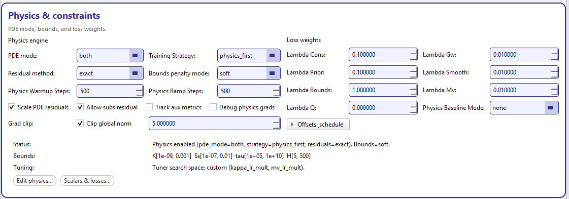
Physics & constraints: core physics engine switches (left), loss weights (right), and a footer summary that makes the current physics state explicit.
Physics engine (left panel)
This panel defines how the physics part of the objective is formed.
- PDE mode
Select which physics residuals are active. Typical values include:
off: no PDE residuals (data losses only)consolidation: enable consolidation residualgroundwater: enable groundwater-flow residualboth: enable consolidation + groundwater residuals
The footer Status line makes this explicit (for example:
Physics enabled (pde_mode=both, strategy=physics_first, residuals=exact).).
- Training strategy
Controls how training balances data-fitting and physics regularization. A common choice is
physics_first: physics is emphasized early, then the model transitions toward balanced optimization (in combination with warmup and ramp steps).- Residual method
Chooses how PDE residuals are computed (e.g.,
exact). This is where the implementation decides whether to use exact autodiff residuals, approximations, or reduced forms.- Bounds penalty mode
Controls how violations of physical bounds are penalized:
soft: add a smooth penalty for out-of-range values(other modes may exist depending on your schema)
- Warmup / ramp steps
These are the two most important “stability” knobs for physics training:
Physics warmup steps (
physics_warmup_steps): number of initial steps/iterations where physics is introduced gently.Physics ramp steps (
physics_ramp_steps): number of steps over which physics weight is ramped toward its target.
These are designed to reduce early-training instability (common in PINNs when physics constraints are too strong before the network has learned basic signal).
The checkbox row enables additional physics-related diagnostics and behaviors:
- Scale PDE residuals
Normalizes residual magnitudes to improve comparability across terms (often recommended when mixing multiple PDE losses).
- Allow subs residual
Enables a subsidence-related residual contribution (when available).
- Track aux metrics
Enables additional diagnostics during training (useful for debugging physics contributions and reporting).
- Debug physics grads
Enables verbose gradient-level debugging for physics terms (intended for development and troubleshooting rather than routine training).
The Grad clip controls expose an optional global norm clipping:
Check Clip global norm to activate clipping.
Set the numeric threshold (
clip_global_norm).
This is one of the most practical tools to prevent exploding gradients when physics terms dominate, especially during early ramp-up.
Loss weights (right panel)
This panel sets the scalar multipliers for each loss component. These values directly control how much each term influences optimization.
- Lambda Cons (
lambda_cons) Weight for consolidation residual loss.
- Lambda Gw (
lambda_gw) Weight for groundwater-flow residual loss.
- Lambda Prior (
lambda_prior) Weight for prior consistency (how strongly learned fields adhere to priors).
- Lambda Smooth (
lambda_smooth) Weight for smoothness regularization (spatial smoothness of fields).
- Lambda Bounds (
lambda_bounds) Weight for bounds penalties (only meaningful when bounds mode is enabled).
- Lambda Mv (
lambda_mv) Weight for additional stabilization/regularization terms (model-variant).
- Lambda Q (
lambda_q) Weight for quantile/probabilistic objective components (when probabilistic outputs are enabled).
- Physics baseline mode (
physics_baseline_mode) Selects an optional baseline reference for physics terms (e.g.,
none). This is useful when you want physics losses computed relative to a baseline rather than absolute magnitudes.
Offsets & schedule (expander)
The Offsets & schedule expander controls a secondary mechanism often used to stabilize training when multiple loss scales compete.
Inside the expander you can configure:
- Offset mode (
offset_mode) Strategy used to compute/interpret the offset.
- Lambda offset (
lambda_offset) Scalar weight for the offset term.
- Use scheduler
When enabled (
use_lambda_offset_scheduler), GeoPrior will schedule the offset weight over time using:lambda_offset_warmup (steps before scheduling begins),
lambda_offset_start (initial value),
lambda_offset_end (final value).
This provides a controlled way to introduce or phase out offset regularization during long runs.
Where to document “Edit physics…” and “Scalars & losses…”
This Setup card is the quick control surface, but the detailed meaning of physics parameters and loss decompositions is most useful in the Train documentation, because that is where users feel the impact (stability, convergence, metrics, and trade-offs).
Recommended placement in your docs tree:
workflow/train_tab.rst: reference this card and explain common presets (data-only vs physics-first vs balanced).workflow/train_tab.rst(orcomponents/physics_and_losses.rst): add dedicated subsections:Edit physics…dialog: describe the full physics schema, priors, bounds, closures, and diagnostics.Scalars & losses…dialog: document the scalar multipliers, search-space ranges for tuning, sampling modes (linear/log), and best practices.
This keeps the Setup tab readable while still giving advanced users a complete, auditable reference for physics configuration.
Other sections
Other cards (architecture, training, physics, probabilistic outputs, tuning, device/runtime, UI preferences) are designed to be edited when you move beyond a minimal run. In early experiments, you can keep these at defaults and focus on paths + time window + semantics.
Search and section filtering
Use the search box in the header to filter sections. Filtering hides non-matching cards and updates the navigation to keep only visible sections. This is the fastest way to jump to a control when you already know its category (e.g., type “epsg”, “horizon”, “gwl”, “lambda”, “heads”, “quantiles”).
Saving your setup (recommended)
Once your run configuration is stable, save a snapshot:
Click Save as (or Save if a path is already set),
store the JSON alongside your results archive or in a separate experiment registry folder.
Saved snapshots make it easy to reproduce experiments, compare runs, and audit exactly what changed.
See also
Preprocess tab (Stage-1) for Stage-1 preprocessing
Train tab and Inference tab for Stage-2 runs
Output folders and file layout for output directory layout
Configuration key reference for a key-level reference