Exercise: Advanced Quantile Forecasting with XTFT
Welcome to this exercise on advanced time series forecasting using
the XTFT (Extreme Temporal Fusion Transformer)
model from fusionlab-learn. XTFT is designed for complex scenarios,
handling static, dynamic past, and known future features to produce
multi-horizon quantile forecasts.
Learning Objectives:
Understand the data preparation steps for XTFT, including feature definition and sequence generation.
Learn how to instantiate, compile, and train an XTFT model for quantile forecasting using all three input types (static, dynamic, future).
Practice making multi-step predictions and interpreting the quantile outputs.
Visualize probabilistic forecasts to understand prediction uncertainty.
Let’s begin!
Prerequisites
Ensure you have fusionlab-learn and its common dependencies
installed. For visualizations, matplotlib is also needed.
pip install fusionlab-learn matplotlib scikit-learn joblib
Step 1: Imports and Setup
First, we import all necessary libraries.
 1import numpy as np
 2import pandas as pd
 3import tensorflow as tf
 4import matplotlib.pyplot as plt
 5from sklearn.model_selection import train_test_split
 6from sklearn.preprocessing import StandardScaler, LabelEncoder
 7import os
 8import joblib
 9import warnings
10
11# FusionLab imports
12from fusionlab.nn.transformers import XTFT
13from fusionlab.nn.utils import reshape_xtft_data
14from fusionlab.nn.losses import combined_quantile_loss
15from fusionlab.datasets.make import make_multi_feature_time_series
16
17warnings.filterwarnings('ignore')
18os.environ['TF_CPP_MIN_LOG_LEVEL'] = '2'
19tf.get_logger().setLevel('ERROR')
20if hasattr(tf, 'autograph'):
21    tf.autograph.set_verbosity(0)
22
23exercise_output_dir_xtft = "./xtft_advanced_exercise_outputs"
24os.makedirs(exercise_output_dir_xtft, exist_ok=True)
25print("Libraries imported for XTFT exercise.")
Expected Output 1.1:
Libraries imported for XTFT exercise.
Step 2: Generate Synthetic Time Series Data
We use make_multi_feature_time_series()
to generate data with static, dynamic, and future features.
 1n_items_ex = 3
 2n_timesteps_ex = 36
 3rng_seed_ex = 42
 4np.random.seed(rng_seed_ex)
 5
 6# Generate data using the fusionlab utility
 7data_bunch_ex = make_multi_feature_time_series(
 8    n_series=n_items_ex,
 9    n_timesteps=n_timesteps_ex,
10    freq='MS', # Monthly data
11    seasonality_period=12, # Yearly seasonality
12    seed=rng_seed_ex,
13    as_frame=False # Get Bunch object to access feature lists
14)
15df_raw_ex = data_bunch_ex.frame.copy() # Work with a copy
16
17print(f"Generated raw data shape for exercise: {df_raw_ex.shape}")
18print(f"Columns: {df_raw_ex.columns.tolist()}")
19print("Sample of generated data:")
20print(df_raw_ex.head(3))
- Expected Output 2.2:
(Shape and sample data will be consistent due to random seed. Column names will match those from `make_multi_feature_time_series`)
Generated raw data shape for exercise: (108, 9)
Columns: ['date', 'series_id', 'base_level', 'month', 'dayofweek', 'dynamic_cov', 'target_lag1', 'future_event', 'target']
Sample of generated data:
     date  series_id  base_level  ...  dayofweek  dynamic_cov     target
0 2020-01-01 0 50.049671 … 2 -0.069132 63.055435 1 2020-02-01 0 50.049671 … 5 0.841482 68.394497 2 2020-03-01 0 50.049671 … 6 1.761515 70.075474
[3 rows x 9 columns]
Step 3: Define Feature Roles and Scale Numerical Data
We use the feature lists provided by data_bunch_ex. Numerical features are scaled. series_id is already numerical.
 1target_col_ex = data_bunch_ex.target_col
 2dt_col_ex = data_bunch_ex.dt_col
 3# Use feature lists from data_bunch
 4static_cols_ex = data_bunch_ex.static_features
 5dynamic_cols_ex = data_bunch_ex.dynamic_features
 6future_cols_ex = data_bunch_ex.future_features
 7spatial_cols_ex = [data_bunch_ex.spatial_id_col]
 8
 9scalers_ex = {}
10# Define numerical columns to scale (excluding IDs and time components
11# that might be treated as categorical by the model's embeddings)
12num_cols_to_scale_ex = ['base_level', 'dynamic_cov', 'target_lag1', target_col_ex]
13# Ensure 'month' and 'dayofweek' are not scaled if they are to be embedded
14# or treated as categorical by the model.
15
16df_scaled_ex = df_raw_ex.copy()
17for col in num_cols_to_scale_ex:
18    if col in df_scaled_ex.columns:
19        scaler = StandardScaler()
20        df_scaled_ex[col] = scaler.fit_transform(df_scaled_ex[[col]])
21        scalers_ex[col] = scaler
22        print(f"Scaled column: {col}")
23    else:
24        print(f"Warning: Column '{col}' for scaling not found in DataFrame.")
25
26scalers_path_ex = os.path.join(
27    exercise_output_dir_xtft, "xtft_exercise_scalers.joblib"
28    )
29joblib.dump(scalers_ex, scalers_path_ex)
30print(f"\nScalers saved to {scalers_path_ex}")
Expected Output 3.3:
Scaled column: base_level
Scaled column: dynamic_cov
Scaled column: target_lag1
Scaled column: target

Scalers saved to ./xtft_advanced_exercise_outputs/xtft_exercise_scalers.joblib
Step 4: Prepare Sequences using reshape_xtft_data
Now, we use the static_cols_ex (which includes series_id and base_level) when calling reshape_xtft_data. This will ensure static_data_ex has features.
 1time_steps_ex = 12
 2forecast_horizons_ex = 6
 3
 4# `static_cols_ex` from data_bunch is ['series_id', 'base_level']
 5# Both are numerical and can be used as static features.
 6static_data_ex, dynamic_data_ex, future_data_ex, target_data_ex = \
 7    reshape_xtft_data(
 8        df=df_scaled_ex,
 9        dt_col=dt_col_ex,
10        target_col=target_col_ex,
11        dynamic_cols=dynamic_cols_ex,
12        static_cols=static_cols_ex, # Use actual static features
13        future_cols=future_cols_ex,
14        spatial_cols=spatial_cols_ex, # Group by 'series_id'
15        time_steps=time_steps_ex,
16        forecast_horizons=forecast_horizons_ex,
17        verbose=1
18    )
- Expected Output 4.4:
(Shapes will reflect actual static features being used)
[INFO] Reshaping time‑series data into rolling sequences...

[INFO] Data grouped by ['series_id'] into 3 groups.

[INFO] Total valid sequences to be generated: 57

[INFO] Final data shapes after reshaping:
  [DEBUG] Static Data : (57, 2)
  [DEBUG] Dynamic Data: (57, 12, 4)
  [DEBUG] Future Data : (57, 18, 3)
  [DEBUG] Target Data : (57, 6, 1)

[INFO] Time‑series data successfully reshaped into rolling sequences.
Step 5: Train/Validation Split of Sequences
Split the generated sequence arrays.
 1val_split_fraction_ex = 0.2
 2if target_data_ex is None or target_data_ex.shape[0] == 0:
 3    raise ValueError("No sequences generated.")
 4
 5n_samples_ex = target_data_ex.shape[0]
 6split_idx_ex = int(n_samples_ex * (1 - val_split_fraction_ex))
 7
 8X_s_train, X_s_val = static_data_ex[:split_idx_ex], static_data_ex[split_idx_ex:]
 9X_d_train, X_d_val = dynamic_data_ex[:split_idx_ex], dynamic_data_ex[split_idx_ex:]
10X_f_train, X_f_val = future_data_ex[:split_idx_ex], future_data_ex[split_idx_ex:]
11y_t_train, y_t_val = target_data_ex[:split_idx_ex], target_data_ex[split_idx_ex:]
12
13train_inputs_ex = [X_s_train, X_d_train, X_f_train]
14val_inputs_ex = [X_s_val, X_d_val, X_f_val]
15
16print(f"\nData split into Train/Validation sequences:")
17print(f"  Train samples: {X_d_train.shape[0]}")
18print(f"  Validation samples: {X_d_val.shape[0]}")
19print(f"  Train Static Shape : {X_s_train.shape}")
20print(f"  Train Dynamic Shape: {X_d_train.shape}")
21print(f"  Train Future Shape : {X_f_train.shape}")
22print(f"  Train Target Shape : {y_t_train.shape}")
Expected Output 5.5:
Data split into Train/Validation sequences:
  Train samples: 45
  Validation samples: 12
  Train Static Shape : (45, 2)
  Train Dynamic Shape: (45, 12, 4)
  Train Future Shape : (45, 18, 3)
  Train Target Shape : (45, 6, 1)
Step 6: Define XTFT Model for Quantile Forecast
Instantiate XTFT. static_input_dim will now
be greater than 0. Explicitly set anomaly_detection_strategy=None.
 1quantiles_ex = [0.1, 0.5, 0.9]
 2output_dim_ex = 1
 3
 4s_dim_ex = X_s_train.shape[-1] # Will be > 0 now
 5d_dim_ex = X_d_train.shape[-1]
 6f_dim_ex = X_f_train.shape[-1]
 7
 8model_ex = XTFT(
 9    static_input_dim=s_dim_ex,
10    dynamic_input_dim=d_dim_ex,
11    future_input_dim=f_dim_ex,
12    forecast_horizon=forecast_horizons_ex,
13    quantiles=quantiles_ex,
14    output_dim=output_dim_ex,
15    embed_dim=16, lstm_units=32, attention_units=16,
16    hidden_units=32, num_heads=2, dropout_rate=0.1,
17    max_window_size=time_steps_ex, memory_size=20,
18    scales=None,
19    anomaly_detection_strategy=None, # Explicitly disable
20    anomaly_loss_weight=0.0
21)
22print("\nXTFT model instantiated (anomaly detection disabled).")
Step 7: Compile and Train the Model
(This step remains the same as in the previous version of the artifact)
 1loss_fn_ex = combined_quantile_loss(quantiles=quantiles_ex)
 2model_ex.compile(
 3    optimizer=tf.keras.optimizers.Adam(learning_rate=0.005),
 4    loss=loss_fn_ex
 5    )
 6print("XTFT model compiled with combined quantile loss.")
 7
 8# Dummy call to build model (optional)
 9try:
10    dummy_s_ex = tf.zeros((1, s_dim_ex)) # s_dim_ex > 0
11    dummy_d_ex = tf.zeros((1, time_steps_ex, d_dim_ex))
12    dummy_f_ex = tf.zeros((1, time_steps_ex + forecast_horizons_ex, f_dim_ex))
13    # model_ex([dummy_s_ex, dummy_d_ex, dummy_f_ex]) # Build
14    # model_ex.summary(line_length=90)
15except Exception as e:
16    print(f"Model build/summary failed: {e}")
17
18print("\nStarting XTFT model training (few epochs for demo)...")
19history_ex = model_ex.fit(
20    train_inputs_ex, y_t_train,
21    validation_data=(val_inputs_ex, y_t_val),
22    epochs=3, batch_size=4, verbose=1 # Reduced for gallery speed
23)
24print("Training finished.")
25if history_ex and history_ex.history.get('val_loss'):
26    val_loss = history_ex.history['val_loss'][-1]
27    print(f"Final validation loss (quantile): {val_loss:.4f}")
Expected Output 7:
XTFT model compiled with combined quantile loss.

Starting XTFT model training (few epochs for demo)...
Epoch 1/3
12/12 [==============================] - 8s 86ms/step - loss: 0.3010 - val_loss: 0.4640
Epoch 2/3
12/12 [==============================] - 0s 8ms/step - loss: 0.1919 - val_loss: 0.5092
Epoch 3/3
12/12 [==============================] - 0s 9ms/step - loss: 0.1450 - val_loss: 0.4088
Training finished.
Final validation loss (quantile): 0.4088
Step 8: Make Predictions and Inverse Transform
(This step remains the same as in the previous version of the artifact)
 1print("\nMaking quantile predictions on validation set...")
 2predictions_scaled_ex = model_ex.predict(val_inputs_ex, verbose=0)
 3print(f"Scaled prediction output shape: {predictions_scaled_ex.shape}")
 4
 5target_scaler_ex = scalers_ex.get(target_col_ex)
 6if target_scaler_ex is None:
 7    print("Warning: Target scaler not found. Plotting scaled values.")
 8    predictions_final_ex = predictions_scaled_ex
 9    y_val_final_ex = y_t_val
10else:
11    num_val_samples_ex = X_s_val.shape[0]
12    num_quantiles_ex = len(quantiles_ex)
13    if output_dim_ex == 1:
14        pred_reshaped_ex = predictions_scaled_ex.reshape(-1, num_quantiles_ex)
15        predictions_inv_ex = target_scaler_ex.inverse_transform(pred_reshaped_ex)
16        predictions_final_ex = predictions_inv_ex.reshape(
17            num_val_samples_ex, forecast_horizons_ex, num_quantiles_ex
18        )
19        y_val_reshaped_ex = y_t_val.reshape(-1, output_dim_ex)
20        y_val_inv_ex = target_scaler_ex.inverse_transform(y_val_reshaped_ex)
21        y_val_final_ex = y_val_inv_ex.reshape(
22            num_val_samples_ex, forecast_horizons_ex, output_dim_ex
23        )
24        print("Predictions and actuals inverse transformed.")
25    else:
26        print("Multi-output inverse transform not shown, plotting scaled.")
27        predictions_final_ex = predictions_scaled_ex
28        y_val_final_ex = y_t_val
Expected Output 8:
Making quantile predictions on validation set...
Scaled prediction output shape: (12, 6, 3)
Predictions and actuals inverse transformed.
Step 9: Visualize Forecast for One Item
(This step remains the same. The visualization will now use the actual `X_val_static` to identify the item, as it contains features.)
 1sample_to_plot_idx_ex = 0 # Plot the first validation sequence's forecast
 2
 3if y_val_final_ex is not None and predictions_final_ex is not None and \
 4   len(y_val_final_ex) > sample_to_plot_idx_ex:
 5    actual_vals_item_ex = y_val_final_ex[sample_to_plot_idx_ex, :, 0]
 6    pred_quantiles_item_ex = predictions_final_ex[sample_to_plot_idx_ex, :, :]
 7    forecast_steps_axis_ex = np.arange(1, forecast_horizons_ex + 1)
 8
 9    # Get the ItemID for the plotted sample from X_val_static
10    # Assuming 'series_id' is the first column in static_cols_ex
11    item_id_plotted = X_s_val[sample_to_plot_idx_ex, 0]
12    # If 'series_id' was label encoded, you might want to inverse_transform it here
13    # For this example, make_multi_feature_time_series provides integer series_id
14
15    plt.figure(figsize=(12, 6))
16    plt.plot(forecast_steps_axis_ex, actual_vals_item_ex,
17             label='Actual Sales', marker='o', linestyle='--')
18    plt.plot(forecast_steps_axis_ex, pred_quantiles_item_ex[:, 1],
19             label='Median Forecast (q=0.5)', marker='x')
20    plt.fill_between(
21        forecast_steps_axis_ex,
22        pred_quantiles_item_ex[:, 0], pred_quantiles_item_ex[:, 2],
23        color='gray', alpha=0.3,
24        label='Prediction Interval (q=0.1 to q=0.9)'
25    )
26    plt.title(f'XTFT Quantile Forecast (Item ID from Static: {item_id_plotted:.0f}, Sample {sample_to_plot_idx_ex})')
27    plt.xlabel('Forecast Step into Horizon')
28    plt.ylabel(f'{target_col_ex} (Units after Inverse Transform if applied)')
29    plt.legend(); plt.grid(True); plt.tight_layout()
30    fig_path_ex = os.path.join(
31        exercise_output_dir_xtft,
32        "exercise_advanced_xtft_quantile_forecast.png"
33        )
34    # plt.savefig(fig_path_ex) # Uncomment to save
35    # print(f"\nPlot saved to {fig_path_ex}")
36    plt.show()
37else:
38    print("\nSkipping plot: Not enough data or predictions missing.")
Example Output Plot:
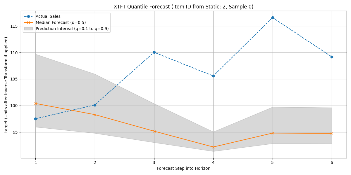
Visualization of the XTFT quantile forecast (median and interval) against actual validation data for a sample item.
Discussion of Exercise:
This exercise walked through a complete workflow for using the
XTFT model for multi-step quantile
forecasting using all three input types: static, dynamic, and future
features. Key takeaways include:
The use of
make_multi_feature_time_series()to generate rich synthetic data.The importance of defining feature roles and appropriately scaling numerical inputs.
Ensuring that static features (like series_id and base_level from make_multi_feature_time_series) are included when calling
reshape_xtft_data()if they are to be used by the model. This results in static_input_dim > 0.Configuring XTFT for quantile output and using
combined_quantile_loss().The ability to inverse-transform predictions for interpretation.
Visualizing quantile forecasts to assess prediction uncertainty.
For real-world applications, extensive hyperparameter tuning (see ../hyperparameter_tuning/index) and more sophisticated validation strategies would be necessary.